
The pursuit of efficient and precise finishing methods for hardened gear teeth represents a significant challenge in modern gear manufacturing, particularly for complex geometries like hyperboloid gears and spiral bevel gears. Grinding, while capable of high accuracy, is often characterized by prohibitive costs and limited availability of specialized machine tools. This article, drawing from extensive research and practical application, presents a detailed examination of skiving—a hard finishing process utilizing carbide cutters with large negative rake angles—as a viable and often superior alternative to grinding for many applications. The core of this analysis lies in the precise mathematical modeling of the skiving cutter’s generating surface and the subsequent calculation methodology required for accurate machine settings, enabling the controlled generation of high-quality tooth flanks on hyperboloid gears.
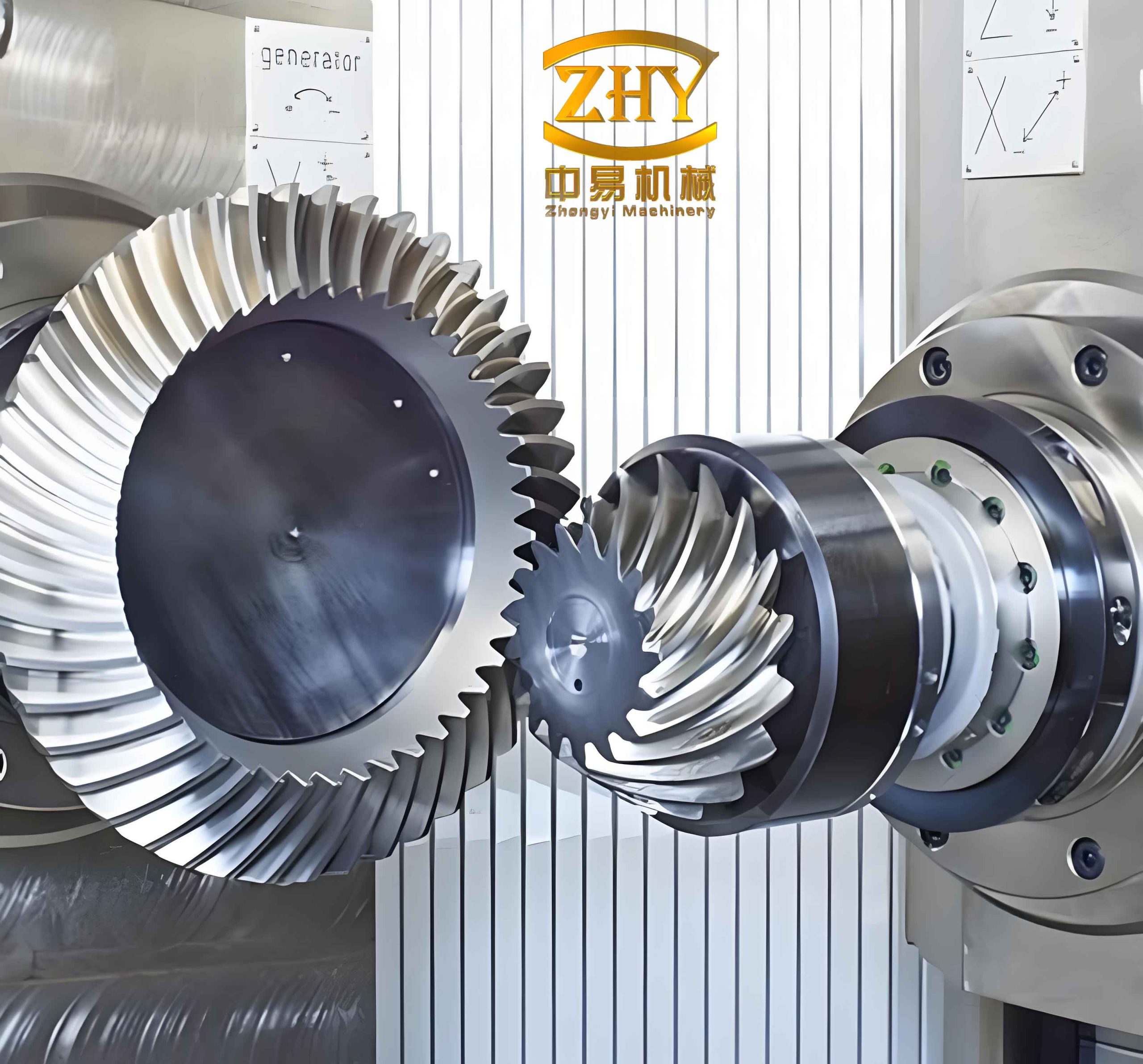
The fundamental geometry of hyperboloid gears involves non-parallel, non-intersecting axes, leading to a complex localized point contact between the pinion and gear teeth. This contact must be carefully controlled to ensure optimal load distribution, low noise, and high durability. The finishing process is critical in establishing this contact pattern. Traditional high-speed steel (HSS) cutters generate a tooth flank via a conical generating surface. Skiving, however, employs carbide inserts with straight cutting edges that are mounted on the cutter head with a significant negative inclination angle, denoted as $\lambda_G$. This simple geometric change—tilting the cutting edge—profoundly alters the kinematics and the generating geometry of the process, transitioning from a simple conical surface to a complex hyperboloidal surface of one sheet. The primary advantage of this setup is the ability to perform “wipe” or “skive” cutting on hardened steel, combining the material removal efficiency of a cutting process with the ability to finish hard teeth.
1. The Generating Surface of the Skiving Cutter
The derivation of the skiving cutter’s generating surface begins with the geometry of the conventional HSS cutter. For a standard cutter, the generating surface at the theoretical cutting point M is a cone with a blade angle $\alpha$. The vector $\vec{MP}$ is defined as $b$. When we introduce the negative inclination $\lambda_G$, the straight cutting edge is no longer contained within this original conical surface but is instead tangent to it at point M. To mathematically describe this, we establish two coordinate systems: $\Sigma$, fixed to the cutter body with its $k$-axis along the original cone axis, and $\Sigma_n$, attached to the cutting edge itself.
In the $\Sigma_n$ system, the equation of the straight cutting edge is simple:
$$
\vec{r_c}^{(n)} = (0, a \sin \lambda_G, -a \cos \lambda_G)^T
$$
where $a$ is a parameter along the cutting edge.
Transforming this into the main coordinate system $\Sigma$ yields:
$$
\vec{r_c} = \begin{pmatrix}
r_{cx} \\
r_{cy} \\
r_{cz}
\end{pmatrix} = \begin{pmatrix}
R_c – (b – a \cos \lambda_G) \sin \alpha \\
a \cos \lambda_G \\
(b – a \cos \lambda_G) \cos \alpha
\end{pmatrix}
$$
Here, $R_c$ is the cutter point radius (the radius to the theoretical cutter tip P). The parameter $b$ is derived from the standard gear generation calculations for the workpiece.
The crucial step is recognizing that this inclined straight line, when rotated around the cutter axis ($k$-axis), does not generate a cone but a one-sheet hyperboloid. Introducing the rotation angle $\theta$ as the second parameter, the equation of the skiving cutter’s generating surface becomes:
$$
\vec{r_d}(a, \theta) = \begin{pmatrix}
\sqrt{r_{cx}^2 + r_{cy}^2} \cdot \cos \theta \\
\sqrt{r_{cx}^2 + r_{cy}^2} \cdot \sin \theta \\
r_{cz}
\end{pmatrix}
$$
This surface $\vec{r_d}(a, \theta)$ is the generating hyperboloid for the skiving process of hyperboloid gears.
2. Curvature Analysis at the Calculation Point
Controlling the contact pattern on the finished hyperboloid gear tooth requires precise knowledge of the surface curvatures at the designated calculation point (often, but not exclusively, the mid-point of the tooth). Therefore, we must analyze the differential geometry of this hyperboloidal generating surface at point M, where $a=0$ and $\theta=0$.
The partial derivatives $\vec{r_d}_a$ and $\vec{r_d}_{\theta}$ are first computed. The unit normal vector $\vec{n}$ to the generating surface at any point is given by:
$$
\vec{n} = \frac{\vec{r_d}_a \times \vec{r_d}_{\theta}}{\sqrt{EG – F^2}}
$$
where $E, F, G$ are the coefficients of the first fundamental form. At the specific calculation point M, this simplifies remarkably to:
$$
\vec{n}_M = \begin{pmatrix}
\cos \alpha \\
0 \\
\sin \alpha
\end{pmatrix}
$$
This is identical to the normal vector of the original conical surface at M. This confirms that although the global surfaces are different (hyperboloid vs. cone), they share a common tangent plane at the calculation point. This is a vital result as it allows us to leverage existing, well-understood calculations for the gear tooth normal and tangent vectors from conventional theory.
The principal curvatures of the generating surface at M must be determined. From differential geometry, the lines of curvature on a one-sheet hyperboloid of revolution are its meridians (hyperbolas) and parallels (circles). The direction of the cutting edge itself is an asymptotic direction on the hyperboloid, meaning the normal curvature in that direction is zero. Using Euler’s formula and Meusnier’s theorem, the two principal curvatures at M can be derived:
- Principal Curvature $k_1$ (Circle Direction): This is found from the circular cross-section (parallel).
$$ k_1 = -\frac{\cos \alpha}{R_c – b \sin \alpha} $$ - Principal Curvature $k_2$ (Hyperbola Direction): This is found using Euler’s formula, knowing the normal curvature is zero in the cutting edge (asymptotic) direction.
$$ k_2 = \frac{\tan^2 \lambda_G \cos \alpha}{R_c – b \sin \alpha} $$
The Gaussian curvature $K$ and Mean curvature $H$ at point M are therefore:
$$ K = k_1 k_2 = -\frac{\tan^2 \lambda_G \cos^2 \alpha}{(R_c – b \sin \alpha)^2} $$
$$ H = \frac{1}{2}(k_1 + k_2) = \frac{\cos \alpha (\tan^2 \lambda_G – 1)}{2(R_c – b \sin \alpha)} $$
The negative Gaussian curvature confirms the surface is hyperbolic (saddle-shaped) at that point, which is characteristic of a one-sheet hyperboloid.
| Property | Conventional HSS Cutter | Skiving Cutter (Carbide) |
|---|---|---|
| Generating Surface | Right Circular Cone | One-Sheet Hyperboloid of Revolution |
| Cutting Edge | Lies on cone surface | Straight line tangent to cone at M, inclined by $\lambda_G$ |
| Surface Type at M | Elliptic ($K > 0$) | Hyperbolic ($K < 0$) |
| Key Design Parameter | Blade Angle ($\alpha$), Point Radius ($R_c$) | Blade Angle ($\alpha$), Point Radius ($R_c$), Inclination Angle ($\lambda_G$) |
| Mathematical Complexity | Lower | Higher (requires hyperboloid geometry) |
3. The Complete Skiving Calculation Methodology for Hyperboloid Gears
The calculation process for skiving hyperboloid gears integrates the new cutter model into the established framework of gear generation theory. The goal is to determine the correct machine settings (cradle angle, sliding base, machine root angle, etc.) and, most importantly, the required skiving cutter parameters to produce a desired tooth contact pattern on the hardened gear.
The step-by-step procedure is as follows:
- Gear Pair Design & Basic Machine Settings: Start with the standard first-order design of the hyperboloid gear pair, establishing the basic machine settings for generating the gear member (usually using a simulated generating gear). These are largely unchanged from conventional methods.
- Work Gear (Gear Member) Calculation: Using the basic settings and the hyperboloidal generating surface model described above, calculate the first-order and second-order parameters (position, normal vector, principal curvatures, and geodesic torsion) of the gear tooth surface at the prescribed calculation point(s). Baxter’s equations, which relate the curvatures of the generating surface to those of the generated surface through the kinematic roll of the process, are applied here.
- Pinion Tooth Surface Determination: Through the conjugate meshing relationship between the gear and the pinion of the hyperboloid gears set, the corresponding point on the theoretical pinion tooth surface and its first- and second-order parameters are calculated.
- Local Synthesis & Pinion Flank Modification: In practice, the theoretical conjugate contact is modified into a controlled localized bearing pattern through a process called local synthesis. This involves specifying desired second-order contact parameters (principal relative curvatures and the direction of the contact path) at the calculation point. These desired parameters, along with the known gear surface, uniquely determine the required second-order parameters ($k_{xc}, k_{yc}, G_c$) for the pinion tooth surface.
- Skiving Cutter Design for the Pinion: This is the critical step unique to skiving. We now have the required pinion surface curvatures at the point. The skiving cutter for the pinion will also have a hyperboloidal generating surface with its own inclination angle $\lambda_p$. The relationship between the generated pinion surface curvatures and the cutter surface curvatures is governed by the following equation derived from the conditions of induced curvature:
$$ (k_{xc} – k_{xd})(k_{yc} – k_{yd}) = G_c^2 $$
where $k_{xd}, k_{yd}$ are the principal curvatures of the pinion skiving cutter’s surface at the calculation point. For the hyperboloidal cutter, we also have $k_{yd} = -k_{xd} \tan^2 \lambda_p$.
Substituting and solving for the required principal curvature of the pinion cutter ($k_{xd}$) yields:
$$
k_{xd} = \frac{Q \pm \sqrt{Q^2 + 4 \tan^2 \lambda_p \cdot K}}{2 \tan^2 \lambda_p}
$$
where $Q = k_{xc} \tan^2 \lambda_p – k_{yc}$ and $K = k_{xc}k_{yc} – G_c^2$ is the Gaussian curvature of the desired pinion flank at the point. The sign is chosen based on the geometry (convex or concave side) to ensure a physically realizable positive cutter point radius. For the convex side of the pinion, which is typically an elliptical point ($K>0$), the positive root is taken.
- Cutter Point Radius Calculation: Once $k_{xd}$ is determined, the required nominal cutter point radius $R_{cp}’$ for the pinion skiving cutter is found using Meusnier’s theorem:
$$ R_{cp}’ = \frac{\cos \alpha_{bp}}{k_{xd}} – b_p \sin \alpha_{bp} $$
where $\alpha_{bp}$ and $b_p$ are the blade angle and offset parameter for the pinion cutter, derived from standard calculations. This calculated radius $R_{cp}’$ is then rounded to the nearest available standard cutter size $R_{cp}$. - Final Machine Settings: With all cutter parameters ($\alpha_{bp}, \lambda_p, R_{cp}$) now defined, the final machine settings for cutting the pinion member of the hyperboloid gears are computed. These adjustment calculations (e.g., modified roll, tilt) proceed identically to those in conventional face-milling or face-hobbing processes, as the fundamental kinematic relationship between cradle rotation and workpiece rotation remains the same; only the definition of the generating surface has changed.
| Stage | Input Parameters | Calculated Outputs | Governing Equations/Principles |
|---|---|---|---|
| 1. Cutter Surface Model | $R_c, \alpha, b, \lambda_G$ | Hyperboloid equation $\vec{r_d}(a,\theta)$, Principal curvatures $k_1, k_2$ | Surface geometry, Differential geometry (Euler/Meusnier) |
| 2. Gear Generation | Basic machine settings, Cutter surface params | Gear tooth point $\vec{r_g}$, Normal $\vec{n_g}$, Curvatures $(k_{g1}, k_{g2}, \tau_g)$ | Gear generation kinematics, Baxter’s equations |
| 3. Local Synthesis | Desired contact ellipse size & orientation | Required pinion curvatures $k_{xc}, k_{yc}, G_c$ | Conjugate theory, Relative curvature tensors |
| 4. Pinion Cutter Design | $k_{xc}, k_{yc}, G_c, \lambda_p$ | Required cutter curvature $k_{xd}$ | Induced curvature relation: $(k_{xc}-k_{xd})(k_{yc}-k_{yd})=G_c^2$ |
| 5. Final Cutter Spec | $k_{xd}, \alpha_{bp}, b_p$ | Required point radius $R_{cp}’$, Chosen standard $R_{cp}$ | Meusnier’s Theorem: $R_{cp}’ = \frac{\cos \alpha_{bp}}{k_{xd}} – b_p \sin \alpha_{bp}$ |
4. Advantages, Applications, and Comparison with Grinding
The implementation of skiving for hyperboloid gears offers distinct advantages, particularly in the context of medium-to-high volume production of driveline components for automotive, aerospace, and industrial machinery.
Primary Advantages:
- Cost Efficiency: Skiving operations typically have higher metal removal rates than grinding and use durable carbide tooling, leading to lower per-part processing costs.
- Process Flexibility: The cutter geometry (via $\lambda_G$, $R_c$) provides an additional set of design variables to control the contact pattern independently of the basic machine kinematics, offering greater flexibility in optimizing tooth contact for noise and strength.
- Surface Integrity: When properly applied, skiving can produce favorable surface finishes and compressive residual stresses, beneficial for fatigue performance.
- Machine Tool Utilization: It can often be performed on the same hypoid generating machines used for soft-cutting, after a tooling change, minimizing capital investment compared to dedicated grinding machines.
Comparison with Grinding:
| Aspect | Skiving (Hard Cutting) | Grinding |
|---|---|---|
| Material Removal Mechanism | Shear cutting with defined carbide edge | Abrasive grain cutting/ploughing |
| Typical Hardness Range (HRC) | Up to ~60-62 HRC | Up to ~65+ HRC |
| Process Speed | High (higher MRR) | Low to Moderate |
| Tooling/Cost | Carbide inserts (lower cost, regrindable) | Specialized grinding worms/wheels (higher cost) |
| Thermal Impact | Moderate (requires coolant management) | High risk of burn (requires precise control) |
| Geometric Accuracy Potential | Very High | Extremely High |
| Surface Finish | Good to Very Good | Excellent |
| Primary Application Focus | High-volume production, cost-sensitive applications | Ultra-high precision, highest hardness, aerospace |
The choice between skiving and grinding for finishing hyperboloid gears ultimately depends on the production volume, required quality specifications, gear hardness, and available manufacturing infrastructure. Skiving has proven to be a highly effective “bridge” process, filling the gap between soft-cutting and precision grinding.
5. Computational Implementation and Practical Considerations
The successful industrial application of skiving for hyperboloid gears relies on robust software that implements the calculation methodology outlined above. Such a system integrates several modules:
- Geometric Modeler: Handles the definition of the hyperboloidal cutter surface and performs differential geometry calculations.
- Kinematic Simulator: Models the precise motion of the machine tool (cradle, workpiece, cutter head rotation).
- Tooth Contact Analysis (TCA): Simulates the meshing of the pinion and gear under load to predict the contact pattern, transmission error, and stress distribution. This is used to iteratively refine the local synthesis inputs.
- Optimization Routines: Automatically adjusts parameters like the inclination angles ($\lambda_G$, $\lambda_p$), calculation point location, and machine settings to achieve desired TCA results while respecting manufacturing constraints.
Key practical factors that must be accounted for in the model include:
- Cutter Wear and Re-grinding: The model must account for the change in the effective cutter point radius $R_c$ as the carbide inserts are re-sharpened.
- Machine Deflections: Under cutting forces, machine and workpiece deflections can slightly alter the generated geometry. Advanced systems may include empirical or FEA-based compensation.
- Cutting Force Prediction: The large negative rake angle influences cutting forces significantly. Force models help in selecting robust machine parameters and predicting stability.
The fundamental equation set governing the skiving process can be summarized in a consolidated form, linking the desired gear mesh performance to the manufacturing parameters. Let $\mathbf{P}_{mesh}$ represent the set of desired mesh characteristics (contact ellipse semi-axes $a_e, b_e$, orientation $\phi$, transmission error amplitude $\Delta TE$). The synthesis solves for the manufacturing set $\mathbf{M}$, which includes machine settings $\mathbf{S}_{machine}$ and cutter parameters $\mathbf{C}_{skive}$:
$$
\mathbf{M} = \arg \min_{\mathbf{S}_{machine}, \mathbf{C}_{skive}} \left\| \text{TCA}\left( \mathbf{S}_{machine}, \mathbf{C}_{skive} \right) – \mathbf{P}_{mesh} \right\|
$$
subject to:
$$
\mathbf{C}_{skive} = \{ R_c, \alpha, \lambda_G, \ldots \} \quad \text{with} \quad k_{1} = -\frac{\cos \alpha}{R_c – b \sin \alpha}, \quad k_{2} = \frac{\tan^2 \lambda_G \cos \alpha}{R_c – b \sin \alpha}
$$
and the kinematic constraints of the specific generator.
Conclusion
The skiving process represents a sophisticated and economically advantageous method for the hard finishing of hyperboloid gears. Its effectiveness hinges on a precise understanding of the altered generating geometry—the transition from a conical to a hyperboloidal tool surface induced by the inclined carbide cutting edge. The comprehensive calculation methodology presented here, from the derivation of the hyperboloid equation through to the determination of cutter parameters via local synthesis and curvature matching, provides the necessary theoretical foundation for its precise implementation. By modifying the cutter parameter calculation module within existing gear generation software to incorporate these formulas, manufacturers can leverage the benefits of skiving to produce high-quality, durable hyperboloid gear sets with controlled contact patterns at a significantly lower cost than grinding, thereby enhancing the performance and value of a wide range of power transmission systems. The continued development and refinement of these computational models will further solidify skiving’s role as a critical technology in the advanced manufacturing of hyperboloid gears.