
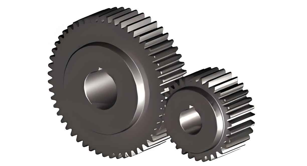
Spur gear transmissions are one of the most widely used power transmission forms in modern machinery owing to their compact structure, high load-carrying capacity, steady transmission ratio and excellent efficiency. As modern equipment moves toward high speed, heavy load and high precision, the vibration of spur gear systems becomes a critical factor affecting reliability, noise and durability. Under realistic operating conditions, spur gear contacts are usually lubricated by an elastohydrodynamic lubrication (EHL) film. The thin lubricating film between meshing tooth surfaces is able to support high contact pressure, and it strongly influences tooth friction and mesh stiffness. In particular, the oil film stiffness and tooth surface friction coefficient are two of the most important internal excitations in a spur gear system. In my study, I focus on the prediction of vibration characteristics of spur gear drives considering EHL effects. I establish a numerical EHL line-contact model, calculate the oil film stiffness and combine it with the gear mesh stiffness, and I also determine the friction coefficient from gearbox power-loss measurements. Then I construct a nonlinear dynamic model of a spur gear pair, investigate the combined effects of friction and stiffness, verify the model with experiments, and finally propose a parallel BP neural network model for fast and reliable prediction of the spur gear vibration response under uncertain parameters.
1 Introduction
Spur gears are fundamental machine elements in automotive, aerospace, marine and industrial applications. With increasing demands for higher power density and lower vibration, a deep understanding of the mechanism that generates gear vibration is necessary. The tooth meshing process is a highly nonlinear interaction in which time-varying mesh stiffness, backlash, transmission error, friction and damping are coupled. When the tooth surfaces are separated by an EHL oil film, the situation becomes even more complex because the oil film itself has stiffness and damping properties, and it changes the friction condition between the surfaces.
Many researchers have studied the dynamics of spur gear systems, and some of them have included EHL oil film stiffness in the dynamic model. It has been shown that the film stiffness can reduce mesh impact and absorb vibration energy. Other works have incorporated tooth friction coefficients into gear dynamic models and found that friction can significantly increase the vibrational response. However, most previous investigations treated oil film stiffness and friction coefficient separately. In real spur gear transmissions, the oil film thickness and the friction coefficient are determined simultaneously by the same lubricated contact. Therefore, it is important to consider the combined effects of the comprehensive mesh stiffness, which includes the oil film stiffness in series with the structural mesh stiffness, and the tooth surface friction coefficient on the vibration response.
Another challenge is that operating conditions vary during service, which makes the oil film thickness, the film stiffness and the friction coefficient uncertain. Traditional gear dynamic models based on Newtonian or analytical mechanics may not be sufficiently fast or flexible when these uncertain parameters vary. In recent years, deep learning methods have become powerful tools for nonlinear regression and pattern recognition. Artificial neural networks, especially BP neural networks, are capable of approximating any continuous nonlinear function and can learn hidden relationships from data. Therefore, I use a parallel BP neural network to predict the vibration characteristics of spur gear drives under uncertain EHL parameters.
2 Elastohydrodynamic Lubrication Model of Spur Gear Contacts
For a spur gear pair, the contact at any meshing instant can be modelled as a line contact between two equivalent cylinders. The equivalent radius of curvature is obtained from the instantaneous radii of curvature of the two tooth profiles. The EHL model is governed by the Reynolds equation, the film thickness equation, the load balance equation and the lubricant rheological equations. In my model, the lubricant is assumed to be Newtonian, the flow is isothermal, and the pressure is constant across the film thickness. The line-contact Reynolds equation can be written as
$$ \frac{\partial}{\partial x}\left(\frac{\rho h^3}{12 \eta}\frac{\partial p}{\partial x}\right) = u_e \frac{\partial (\rho h)}{\partial x} + \frac{\partial (\rho h)}{\partial t}, $$
where \(p\) is the hydrodynamic pressure, \(h\) is the film thickness, \(\rho\) and \(\eta\) are the density and viscosity of the lubricant, \(x\) is the coordinate along the entrainment direction, and \(u_e\) is the entrainment velocity. The boundary conditions are \(p=0\) at the inlet \(x_{in}\), \(p=0\) at the outlet \(x_{out}\), and \(\partial p/\partial x = 0\) at the outlet.
The film thickness equation for the equivalent elastic cylinder is
$$ h(x,t) = h_0(t) + \frac{x^2}{2R} – \frac{2}{\pi E’} \int_{x_{in}}^{x_{out}} p(x’,t) \ln\left(x-x’\right)^2 dx’, $$
where \(h_0(t)\) is the rigid central film thickness, \(R\) is the equivalent radius of curvature, and \(E’\) is the equivalent elastic modulus. The pressure-viscosity relationship is represented by the Roelands equation,
$$ \eta = \eta_0 \exp\left\{ \left(\ln \eta_0 + 9.67\right)\left[\left(1+5.1\times 10^{-9} p\right)^{z_0}-1\right] \right\}, $$
and the density-pressure relationship by the Dowson-Higginson equation,
$$ \rho = \rho_0 \left[ 1 + \frac{0.6\times 10^{-9} p}{1+1.7\times 10^{-9} p} \right]. $$
The load balance condition is
$$ \int_{x_{in}}^{x_{out}} p(x,t) dx = w, $$
where \(w\) is the applied load per unit width. I solved the EHL model using the multigrid method, which provides efficient and stable convergence for the strong nonlinearity. The computational domain was \(X_{in}=-2.5\) to \(X_{out}=1.5\), with five grid levels. The convergence criterion was that the relative pressure error was less than \(10^{-4}\).
2.1 Effect of torque on EHL behavior
I first studied the effect of torque on the oil film pressure and film thickness. The spur gear parameters used in the calculation are listed in Table 1.
| Parameter | Value |
|---|---|
| Lubricant dynamic viscosity \(\eta_0\) (Pa·s) | 0.082 |
| Lubricant density \(\rho_0\) (kg/m³) | 880 |
| Equivalent elastic modulus \(E’\) (Pa) | \(2.2\times10^{11}\) |
| Contact line length \(l\) (mm) | 20 |
| Viscosity-pressure coefficient \(\alpha\) (m²/N) | \(2.19\times10^{-8}\) |
| Equivalent radius \(R\) (mm) | 8 |
| Environmental temperature (°C) | 40 |
At a speed of 1400 r/min, I increased the torque from 50 N·m to 150 N·m and then to 300 N·m. The computed oil film pressure showed that at 50 N·m the pressure distribution was close to the Hertzian dry contact distribution but without a secondary pressure spike. When the torque increased to 150 N·m, a secondary pressure spike appeared. At 300 N·m, the secondary spike became lower and moved toward the outlet. The film thickness decreased with increasing torque. This is because the higher load compresses the film more severely, and the outlet constriction also becomes less pronounced.
2.2 Effect of speed on EHL behavior
At a torque of 150 N·m, I varied the speed from 800 r/min to 1400 r/min, 1800 r/min and 3000 r/min. With increasing speed, the entrainment velocity rose, more lubricant was drawn into the contact, and the film thickness increased. The secondary pressure spike became larger and moved toward the inlet. Compared with torque, speed had a moderate influence on the pressure and film thickness distributions. The computed oil film thickness and pressure were then used to calculate the oil film stiffness.
3 Comprehensive Mesh Stiffness and Tooth Surface Friction Coefficient
3.1 Oil film stiffness and comprehensive mesh stiffness
In EHL line contacts, the oil film acts as a nonlinear spring in the normal direction. The normal oil film stiffness can be calculated from the average film pressure and film thickness. I computed it using a discretized expression based on the numerical pressure and film thickness fields:
$$ K_o = \sum_{i=1}^{n} \frac{p_i}{H_i} \cdot \frac{n l R \Delta X}{b \Delta H}, $$
where \(p_i\) and \(H_i\) are the dimensionless pressure and film thickness at node \(i\), \(n\) is the number of nodes, \(l\) is the contact length, \(R\) is the equivalent radius, \(\Delta X\) is the dimensionless grid spacing, \(b\) is the half-width of the Hertzian contact, and \(\Delta H\) is the film thickness variation. The oil film stiffness changes along the line of action because the load, radii of curvature and entrainment velocity all vary during meshing.
To account for the effect of the lubricating film on the spur gear mesh, I considered the gear mesh stiffness \(K_m\) and the oil film stiffness \(K_o\) as two springs connected in series. The comprehensive mesh stiffness \(K\) is
$$ K = \frac{K_m K_o}{K_m + K_o}. $$
I calculated the time-varying mesh stiffness \(K_m\) with the Weber energy method. In this method, the total mesh compliance is composed of the tooth bending compliance \(\zeta_b\), the local Hertzian contact compliance \(\zeta_c\) and the fillet-foundation compliance \(\zeta_f\). The total deformation of a gear pair at a meshing point is
$$ \zeta_{pg} = \zeta_{bp} + \zeta_{cp} + \zeta_{fp} + \zeta_{bg} + \zeta_{cg} + \zeta_{fg}, $$
and the mesh stiffness is
$$ K_m = \frac{F}{\zeta_{pg}}, $$
where \(F\) is the normal load. Combining the time-varying mesh stiffness with the oil film stiffness yields the comprehensive mesh stiffness used in the dynamic analysis.
3.2 Effect of operating parameters on comprehensive mesh stiffness
I analyzed the influence of torque and speed on the comprehensive mesh stiffness. Table 2 lists the spur gear parameters used in this study.
| Parameter | Driving gear | Driven gear |
|---|---|---|
| Number of teeth | 24 | 16 |
| Module (mm) | 4.5 | 4.5 |
| Pressure angle (°) | 20 | 20 |
| Profile shift coefficient | -0.5 | 0.8532 |
| Face width (mm) | 20 | 20 |
| Density (kg/m³) | \(7.8\times10^3\) | \(7.8\times10^3\) |
| Inner bore diameter (mm) | 30 | 30 |
With increasing torque at a speed of 1400 r/min, the oil film thickness decreased and the oil film became less compressible; therefore, the oil film stiffness increased. The comprehensive mesh stiffness also increased with torque. For example, when the torque increment increased from 100 N·m to 250 N·m, the maximum comprehensive mesh stiffness changed accordingly. With increasing speed at constant torque, the entrainment velocity became larger, producing a thicker oil film. The film became more compliant and the oil film stiffness decreased, which led to a reduction in the comprehensive mesh stiffness.
3.3 Measurement of tooth surface friction coefficient
I measured the tooth surface friction coefficient indirectly from power loss in a back-to-back FZG spur gear test rig. The total gearbox power loss \(P_V\) can be divided into gear friction loss \(P_{VZP}\), no-load loss \(P_{VZ0}\), bearing loss \(P_{VL}\) and seal loss \(P_{VD}\). The gear friction power loss is obtained as
$$ P_{VZP} = P_{V,total} – P_{VZ0,total} – P_{VL,total} – P_{VD,total} – P_{VZP,slave}. $$
The bearing power loss was calculated from the SKF friction torque model:
$$ P_{VL} = M \omega, \quad M = M_{rr} + M_{sl} + M_{seal}, $$
where \(M_{rr}\) is the rolling friction torque, \(M_{sl}\) is the sliding friction torque and \(M_{seal}\) is the seal friction torque. The seal loss was calculated from the Freudenberg equation:
$$ P_{VD} = 7.69 \times 10^{-6} d_{sh}^2 n, $$
where \(d_{sh}\) is the seal diameter and \(n\) is the rotational speed. The tooth surface friction coefficient \(\mu\) is then
$$ \mu = \frac{P_{VZP}}{P_{IN} U_V}, $$
where \(P_{IN}\) is the input power and \(U_V\) is the gear loss factor. In the experiments, the torque loss was measured with a high-precision torque meter at speeds of 400, 800, 1400, 1800, 3000 and 3500 r/min and torques of 5, 50, 150 and 300 N·m. The 5 N·m torque was used to determine the no-load losses. Each operating point was repeated three times.
3.4 Results of friction coefficient measurements
The measured gearbox torque loss increased with speed under no-load conditions because of churning and windage. At a torque of 50 N·m, the torque loss increased from 5.63 N·m to 12.41 N·m when the speed rose from 400 r/min to 3500 r/min. At higher torques of 150 N·m and 300 N·m, the total torque loss first decreased slightly with speed due to improved film formation, and then increased with speed because of the growing no-load losses.
Using the power loss model, I calculated the friction coefficients. Table 3 gives the friction coefficient under several operating conditions.
| Torque (N·m) | Speed (r/min) | Friction coefficient \(\mu\) |
|---|---|---|
| 50 | 1400 | 0.0271 |
| 150 | 1400 | 0.0692 |
| 300 | 1400 | 0.119 |
| 150 | 400 | 0.1505 |
| 150 | 1800 | 0.0554 |
The results show that torque has a stronger influence than speed. At 1400 r/min, the friction coefficient increased from 0.0271 to 0.119 when the torque increased from 50 N·m to 300 N·m, an increase of 339%. The rate of increase became smaller at higher torques. At 150 N·m, the friction coefficient decreased from 0.1505 to 0.0554 when the speed increased from 400 r/min to 1800 r/min, a reduction of 63.2%. This behavior is consistent with the changes in oil film thickness: thicker films separate the surfaces and reduce the friction coefficient, while higher loads produce thinner films and increase asperity interaction.
4 Nonlinear Dynamic Model of Spur Gear Transmission
Based on the calculated comprehensive mesh stiffness and the measured friction coefficient, I established a lumped-parameter dynamic model of a spur gear pair. The model has two rigid gears, each with three degrees of freedom: two translational displacements and one rotation. The gear body is supported by equivalent springs and dampers. The dynamic model includes tooth backlash, time-varying mesh stiffness, viscous mesh damping, transmission error and tooth surface friction. The equations of motion are
$$ m_p \ddot{x}_p + c_{px}\dot{x}_p + k_{px} x_p = F_d \sin\alpha + F_f \cos\alpha, $$
$$ m_p \ddot{y}_p + c_{py}\dot{y}_p + k_{py} y_p = F_d \cos\alpha – F_f \sin\alpha, $$
$$ I_p \ddot{\theta}_p = T_p – F_d r_{bp} – F_f R_p, $$
$$ m_g \ddot{x}_g + c_{gx}\dot{x}_g + k_{gx} x_g = -F_d \sin\alpha – F_f \cos\alpha, $$
$$ m_g \ddot{y}_g + c_{gy}\dot{y}_g + k_{gy} y_g = -F_d \cos\alpha + F_f \sin\alpha, $$
$$ I_g \ddot{\theta}_g = -T_g + F_d r_{bg} + F_f R_g. $$
In these equations, \(m_i\), \(I_i\), \(x_i\), \(y_i\) and \(\theta_i\) are the mass, moment of inertia, horizontal displacement, vertical displacement and rotational displacement of the driving gear \(i=p\) and driven gear \(i=g\), respectively; \(k_{ix}\), \(k_{iy}\), \(c_{ix}\), \(c_{iy}\) are the equivalent support stiffnesses and damping coefficients; \(r_{bi}\) is the base circle radius; \(R_i(t)\) is the instantaneous radius of curvature at the meshing point; \(T_p\) and \(T_g\) are the input and output torques; and \(\alpha\) is the pressure angle.
The gear meshing relative displacement along the line of action is
$$ \delta(t) = (x_p – x_g)\sin\alpha + (y_p – y_g)\cos\alpha + R_p \theta_p – R_g \theta_g – e(t), $$
where \(e(t)\) is the static transmission error. The backlash function is defined as
$$ f(\delta) = \begin{cases} \delta – b_t, & \delta > b_t, \\ 0, & -b_t \le \delta \le b_t, \\ \delta + b_t, & \delta < -b_t, \end{cases} $$
where \(b_t\) is the half-backlash. In this study, the backlash value was taken as 0.05 mm. The dynamic meshing force is
$$ F_d(t) = K(t) f(\delta) + c_m(t) \dot{\delta}, $$
where \(c_m(t)\) is the time-varying mesh damping, which can be related to the mesh stiffness and the gear inertias by
$$ c_m(t) = 2 \xi \sqrt{ \frac{K(t) r_{bp}^2 r_{bg}^2 I_p I_g}{r_{bp}^2 I_p + r_{bg}^2 I_g} }, $$
with the damping ratio \(\xi=0.04\). The friction force on the tooth surface is
$$ F_f(t) = \lambda \mu F_d(t), $$
where \(\lambda\) is the direction sign of friction. The equations were solved by a fourth-order fixed-step Runge-Kutta method. Table 4 gives the mass and moment of inertia values used in the dynamic model.
| Parameter | Driving gear | Driven gear |
|---|---|---|
| Mass (kg) | 1.17 | 0.64 |
| Moment of inertia (kg·m²) | \(1.72\times10^{-3}\) | \(0.58\times10^{-3}\) |
5 Numerical Analysis of Vibration Characteristics
5.1 Influence of comprehensive mesh stiffness
I first investigated the influence of the comprehensive mesh stiffness on the stability of the spur gear system. Using the input speed of 1400 r/min and torque of 300 N·m, I varied the comprehensive mesh stiffness in the range from \(1.1\times10^5\) N/mm to \(2.17\times10^7\) N/mm. The bifurcation diagram showed that the system exhibited a single-period motion for stiffness between \(1.1\times10^5\) N/mm and \(1.731\times10^7\) N/mm. When the stiffness reached \(1.741\times10^7\) N/mm, the motion changed to a quasi-periodic three-period motion, indicating bifurcation. In the range from \(1.741\times10^7\) N/mm to \(1.821\times10^7\) N/mm, the system became multi-periodic. Then, at approximately \(1.831\times10^7\) N/mm, chaotic behavior appeared. When the stiffness exceeded \(1.961\times10^7\) N/mm, the solution diverged. The maximum Lyapunov exponent was negative in the stable region and became positive in the chaotic region, confirming the bifurcation analysis.
These results demonstrate that the oil film stiffness plays a key role in the stability of the spur gear system. Because the oil film is more compliant than the tooth structure, it reduces the total stiffness and allows the system to absorb vibration energy. Therefore, the comprehensive mesh stiffness that accounts for EHL tends to improve the smoothness of meshing and reduce vibration levels.
5.2 Influence of tooth surface friction coefficient
I compared the dynamic response of the spur gear pair for friction coefficients of 0.05, 0.15 and 0.25 at a speed of 1400 r/min and torque of 300 N·m. The time-domain results showed that the steady-state vibration acceleration amplitude increased from about 1.5 m/s² at \(\mu=0.05\) to 1.9 m/s² at \(\mu=0.15\), and further to 2.4 m/s² at \(\mu=0.25\). In the frequency domain, the first mesh-frequency peak increased from 1.4 m/s² to 2.3 m/s². Therefore, a larger friction coefficient leads to stronger frictional excitation and more severe vibration. Higher friction also increases the time required for the system to reach steady state.
5.3 Coupled influence of friction coefficient and comprehensive mesh stiffness
In actual operation, the friction coefficient and the comprehensive mesh stiffness change simultaneously. I simulated the spur gear dynamic response at 1400 r/min with torques of 150, 200 and 300 N·m. As the torque increased, the oil film became thinner, which increased the friction coefficient and also increased the comprehensive mesh stiffness. The numerical results showed that the steady-state vibration acceleration amplitude increased from 3.6 m/s² at 150 N·m to 4.4 m/s² at 200 N·m and 5.6 m/s² at 300 N·m. The peak amplitude at the first mesh frequency also increased from 1.5 m/s² to 2.53 m/s². This means that, in the studied range, the negative effect of increasing friction outweighs the positive stiffness effect.
I also studied the influence of speed at a torque of 300 N·m. When the speed increased from 400 r/min to 800 r/min, the vibration acceleration amplitude decreased from 4.7 m/s² to 4.0 m/s², because the oil film became thicker and the friction coefficient decreased. When the speed increased further from 800 r/min to 1400 r/min, the vibration amplitude remained nearly constant at about 4.1 m/s². The combined effects of decreasing friction and decreasing comprehensive mesh stiffness produced a complex behavior. The phase diagrams showed that the dynamic stability improved from 400 r/min to 800 r/min but worsened from 800 r/min to 1800 r/min. This is because the reduction in friction becomes less dominant at higher speeds, while the reduction in mesh stiffness weakens the system and promotes instability.
6 Experimental Verification
6.1 Test rig and measurement setup
I carried out experiments on an FZG back-to-back spur gear test rig to verify the numerical dynamic model. The rig is driven by a high-speed AC motor and uses a hydraulic loading unit to apply constant torque to the test gear pair. The test gears were the same spur gear pair described in Table 2. The gears were made of 20CrMnTi alloy steel, carburized and hardened to 60-62 HRC. The average surface roughness of the pinion and wheel was 0.35 μm and 0.30 μm, respectively. The pinion and wheel were mounted in the test gearbox and lubricated by an 80W gear oil. The oil temperature was maintained between 35 °C and 45 °C.
The vibration acceleration was acquired using piezoelectric accelerometers mounted on the test gearbox housing. A photoelectric sensor was used to measure the shaft speed. The signals were recorded with a multi-channel data acquisition system. The vibration sensors were placed near the bearing housing in both the radial and axial directions. The test procedures included sweep-speed tests and steady-speed tests. In the sweep test, the torque was kept constant at 20 N·m and the speed was increased continuously from 0 to 3000 r/min and then decreased back to 0. In the steady-speed tests, the speed and torque were set according to the simulation conditions, as shown in Table 5.
| Operating mode | Speed (r/min) | Torque (N·m) |
|---|---|---|
| Low-speed | 400 | 50 |
| Low-speed | 400 | 150 |
| Low-speed | 1400 | 50 |
| Low-speed | 1400 | 150 |
| High-speed | 3500 | 50 |
| High-speed | 3500 | 150 |
6.2 Sweep-speed test results
The sweep test showed that the overall vibration level increased with speed. In the time-frequency spectrogram, the mesh frequency and its harmonics varied with the speed. At high speeds, the vibration energy in the high-frequency band between 3500 Hz and 4500 Hz grew markedly. Order analysis showed that the vibration energy was concentrated around orders 1, 1.5, 2, 2.5, 3 and 3.8. A strong peak in the total energy occurred at 2017 r/min, mainly due to an increase in the 1.5-order component. After 2400 r/min, the third-order component became dominant because it approached a structural resonance frequency. These observations agree with the numerical prediction that increasing speed generally intensifies the spur gear vibration.
6.3 Steady-speed test results and comparison with simulation
For the steady-speed tests, I compared the measured vibration acceleration with the numerical simulation results from the nonlinear dynamic model. The comparisons were performed at speeds of 400 r/min and 1400 r/min with a torque of 150 N·m. Both the time-domain waveforms and the frequency spectra showed good agreement. The dominant peaks occurred at the mesh frequency and its harmonics. The simulation peak frequencies were very close to the measured frequencies. The root-mean-square (RMS) vibration accelerations from the simulation and experiment are compared in Table 6.
| Speed (r/min) | Torque (N·m) | Simulated RMS (m/s²) | Measured RMS (m/s²) | Relative error |
|---|---|---|---|---|
| 400 | 150 | 0.32 | 0.34 | 6.3% |
| 1400 | 150 | 2.37 | 2.60 | 9.7% |
| 3500 | 150 | 41.28 | 42.97 | 4.1% |
For the model without considering the comprehensive mesh stiffness and friction coefficient, the simulated RMS at 1400 r/min and 150 N·m was 2.18 m/s², while the measured value was 2.60 m/s², giving a relative error of 19.3%. The model containing both EHL effects produced an error of 9.7%, which is considerably smaller. Therefore, the proposed dynamic model is more representative of the actual spur gear transmission behavior than the model with dry or simplified contacts.
7 Prediction of Spur Gear Vibration Using BP Neural Network
7.1 Uncertainty quantification of friction coefficient and mesh stiffness
In practice, the friction coefficient and the comprehensive mesh stiffness are affected by fluctuations in load, speed, temperature and lubricant properties. I treated them as random parameters following truncated normal distributions satisfying the \(3\sigma\) rule, with the mean value equal to the calculated average value and the standard deviation equal to 0.83% of the mean. I used bootstrap resampling to estimate the 95% confidence intervals. At each time instant, the friction coefficient and comprehensive mesh stiffness were sampled within their confidence intervals. The uncertainty ranges reflect the realistic dispersion caused by EHL film variations. For example, the friction coefficient at some time instants had a 95% confidence interval from 0.0987 to 0.1031, while the comprehensive mesh stiffness interval was centered near the corresponding calculated value.
7.2 Data generation and preprocessing
To train the prediction model, I generated a dataset from the nonlinear dynamic simulation. The input parameters were the comprehensive mesh stiffness \(K\), the friction coefficient \(\mu\), the backlash function \(f(\delta)\), and the transmission error \(e(t)\). The outputs were the vibration acceleration \(a\) and the dynamic meshing force \(F_d\). The simulation was run for 1 s at a speed of 1400 r/min and a torque of 150 N·m. Data were extracted every 0.01 s, and the process was repeated 100 times with different random samples of the uncertain parameters, generating 10,000 samples. I also generated data along the line of action for the dynamic meshing force to reflect the within-mesh variation.
The dataset was preprocessed by filling missing values with the column mean, removing outliers using the Z-score method, and applying a moving average filter to reduce noise. Because the first 0.2 s contained transient behavior, I excluded those data points. All input and output features were normalized to the range [0,1] using the min-max scaling method:
$$ X_{std} = \frac{X – X_{min}}{X_{max} – X_{min}} (X_{std,max} – X_{std,min}) + X_{std,min}. $$
The dataset was divided into training, validation and test sets in the ratio 8:1:1. The training set was used to update the network weights, the validation set was used to prevent overfitting, and the test set was used only for final evaluation.
7.3 Design of the parallel BP neural network
I designed a parallel BP neural network model (BPNN-PL) consisting of two sub-networks: one for predicting the vibration acceleration and one for predicting the dynamic meshing force. Both sub-networks share the same input variables but are trained separately to optimize their respective output. Each sub-network had two hidden layers. I determined the number of hidden neurons by comparing the mean squared error (MSE) and mean absolute error (MAE) for neuron numbers from 2 to 11. For the vibration acceleration network, 11 hidden neurons gave the best performance. For the dynamic meshing force network, 10 hidden neurons gave the best performance. The activation function between the input layer and the first hidden layer was the tansig function:
$$ \text{tansig}(x) = \frac{2}{1+e^{-2x}} – 1. $$
The activation functions between the hidden layers and the output layer were ReLU functions. The weights and biases were initialized using the default MATLAB neural network toolbox method. The Levenberg-Marquardt algorithm was used for training. The learning rate was set to 0.01 and the maximum number of training epochs was 1200.
7.4 Prediction results and model evaluation
After training, I evaluated the BPNN-PL model on the test set. The predicted values of vibration acceleration and dynamic meshing force were very close to the simulated values. The relative error for most test samples was below 5%. Table 7 summarizes the evaluation metrics.
| Output | MSE | MAE | R² | Average absolute relative error |
|---|---|---|---|---|
| Vibration acceleration | 0.02 | 0.109 | 0.996 | 2.26% |
| Dynamic meshing force (0.01 s interval) | 0.01 | 0.083 | 0.998 | 2.22% |
| Dynamic meshing force (along line of action) | 0.008 | 0.061 | 0.998 | 1.76% |
The high \(R^2\) values close to 1 indicate that the model explains nearly all of the variance in the data and possesses good generalization ability. The small MSE and MAE values show that the prediction accuracy is high. The average absolute relative error below 5% confirms that the BPNN-PL model can reliably predict the vibrational response of the spur gear transmission under uncertain EHL parameters.
7.5 Comparison between prediction and experiment
To further validate the neural network predictor, I compared the predicted vibration acceleration with the experimental measurements under the same operating conditions. The comparison was performed for speeds of 1400 r/min and 3500 r/min under torques of 50 N·m and 150 N·m. The predicted time-domain vibration waveforms agreed well with the measured waveforms in both amplitude and phase characteristics. The RMS vibration accelerations are compared in Table 8.
| Speed (r/min) | Torque (N·m) | Predicted RMS (m/s²) | Measured RMS (m/s²) | Relative error |
|---|---|---|---|---|
| 1400 | 50 | 1.45 | 1.31 | 10.6% |
| 3500 | 50 | 12.65 | 11.81 | 7.1% |
| 1400 | 150 | 2.96 | 2.60 | 13.8% |
| 3500 | 150 | 46.84 | 42.97 | 9.1% |
The relative error is around 10%, which is acceptable for engineering prediction. The remaining error is caused by measurement noise, motor-induced vibrations, unmodelled housing flexibility and the approximate nature of the neural network training data. Overall, the BPNN-PL model provides a fast and reliable method to predict the vibration characteristics of spur gear drives under elastohydrodynamic lubrication.
8 Conclusion
In this work, I studied the vibration characteristics of spur gear drives considering elastohydrodynamic lubrication. The main conclusions are as follows:
(1) The EHL line-contact model was solved with the multigrid method. The oil film pressure and film thickness were strongly affected by torque and speed. Increasing torque reduced the film thickness and changed the secondary pressure spike, while increasing speed increased the film thickness. The oil film stiffness was incorporated into the comprehensive mesh stiffness. The comprehensive mesh stiffness increased with torque and decreased with speed. The tooth surface friction coefficient was measured by the power-loss method. Torque had a stronger influence on the friction coefficient than speed. Increasing torque increased the friction coefficient from 0.0271 to 0.119, while increasing speed reduced it from 0.1505 to 0.0554.
(2) A nonlinear dynamic model of a spur gear pair was developed that includes the comprehensive mesh stiffness, tooth friction, time-varying damping and backlash. The simulation results showed that the oil film stiffness can absorb vibration energy and reduce the vibration amplitude. An increase in the friction coefficient increased the vibrational acceleration and made the system more unstable. Under coupled changes, the friction coefficient had a more significant influence on the spur gear vibration than the comprehensive mesh stiffness.
(3) The dynamic model was verified by experiments on an FZG spur gear test rig. The sweep-speed tests confirmed that increasing speed intensified the vibration. The steady-speed tests showed that the RMS acceleration increased with torque and speed. The numerical results from the proposed model were in good agreement with the measured results, with a maximum RMS relative error of about 10%. The model without EHL effects produced a much larger error, demonstrating the importance of including the oil film stiffness and friction coefficient in the spur gear dynamic model.
(4) A parallel BP neural network model was established to predict the vibration response of the spur gear system under uncertain EHL parameters. The uncertainty of the friction coefficient and the comprehensive mesh stiffness was quantified by confidence intervals. The prediction model achieved MSE values below 0.02, MAE values below 0.11, and \(R^2\) values above 0.996. The average relative error of the predicted outputs was below 5%, and the comparison with experimental data gave RMS errors around 10%. Thus, the proposed neural network model can provide accurate and efficient prediction of spur gear vibration characteristics under elastohydrodynamic lubrication and can be a valuable tool for the design and condition monitoring of spur gear transmissions.