
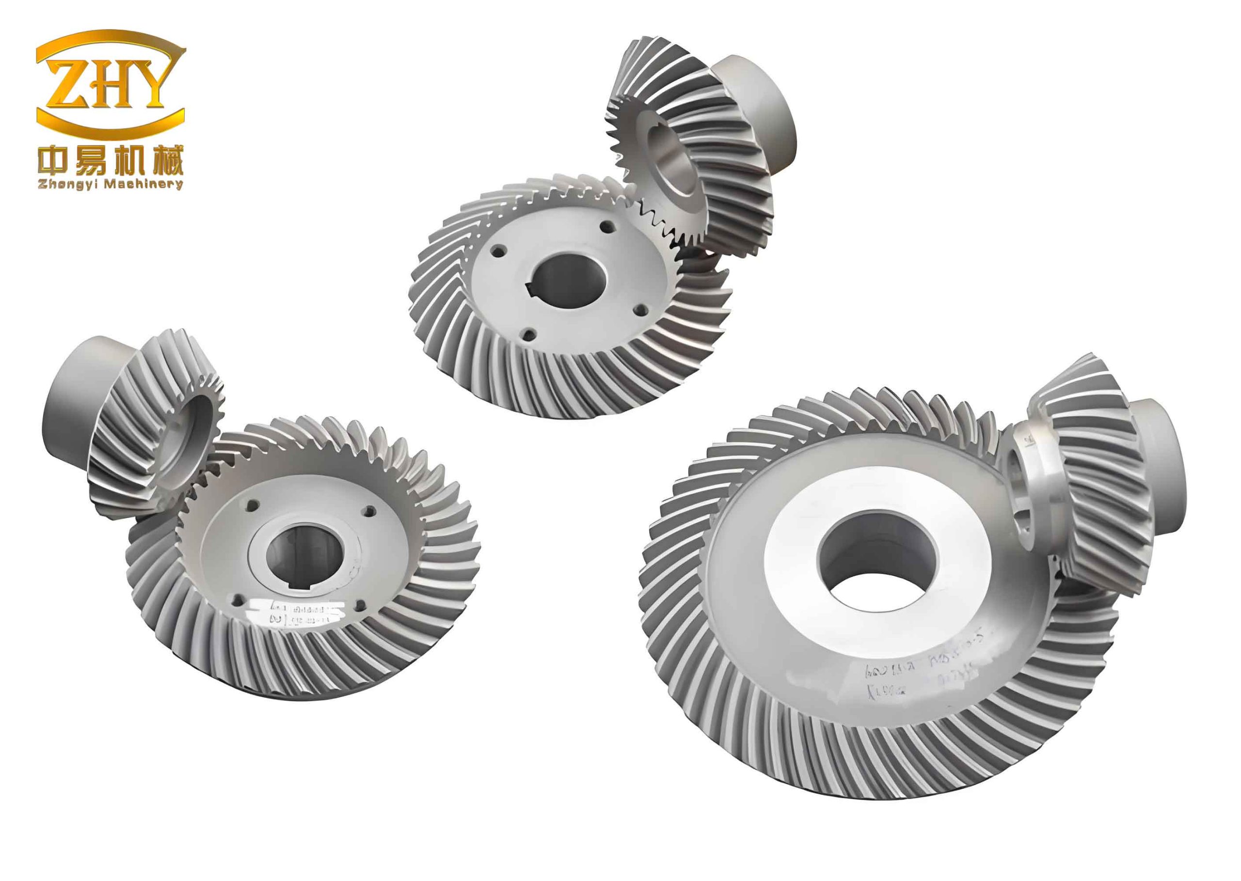
In the realm of automotive powertrains, particularly for commercial vehicles, the drive axle serves as a critical subsystem responsible for transmitting power from the propeller shaft to the driving wheels. At the heart of this transmission lies the gearset, with face-hobbing hyperboloidal gears being a predominant choice due to their superior load-carrying capacity, smooth operation enabled by continuous indexing, and the ability to achieve a lower propeller shaft placement for enhanced vehicle design. The operational demands on these hyperboloidal gears are severe, characterized by high torque transmission and considerable rotational speeds, placing them firmly within the high-speed, heavy-load regime.
Under such demanding conditions, the structural compliance of the entire drive axle system—comprising gears, shafts, rolling-element bearings, and the housing—becomes non-negligible. The resultant system-wide deformation induces misalignments at the gear mesh, deviating from the theoretically ideal contact conditions meticulously designed during manufacture. This misalignment precipitates a skewed load distribution across the tooth flank, leading to localized stress concentrations, accelerated wear, and increased power loss. Consequently, accurately predicting the loaded tooth contact pattern and the associated meshing efficiency is paramount for optimizing gear design, ensuring durability, and improving the overall energy efficiency of the vehicle. Traditional efficiency calculations often treat the gear pair in isolation, neglecting the intricate coupling between system deformation and meshing state. This work, therefore, presents a comprehensive methodology to calculate the meshing efficiency of drive axle hyperboloidal gears by rigorously integrating system deformation effects through a coupled modeling approach.
Theoretical Framework and Methodology
The proposed methodology is built upon a synergistic integration of system-level deformation analysis and detailed gear contact mechanics. The core idea is to first determine the kinematic misalignment of the gear pair caused by the elastic deformation of the entire drive axle under operational loads. This misalignment is then fed into a Frictional Loaded Tooth Contact Analysis (FLTCA) model that operates on the真实的 tooth geometry to compute the pressure distribution and friction forces, ultimately leading to the meshing efficiency.
1. System Deformation and Gear Mesh Misalignment
The drive axle is modeled as a multi-support shaft-bearing-housing coupled system. This model synthesizes the stiffness contributions of all major components: the pinion and gear shafts, the rolling element bearings (modeled with nonlinear stiffness characteristics), the differential housing, and the axle housing itself. The global equilibrium of the system under load is governed by the stiffness equation:
$$ \mathbf{K} \cdot \boldsymbol{\delta} = \mathbf{F} $$
where \(\mathbf{K}\) is the assembled global stiffness matrix of the system, \(\boldsymbol{\delta}\) is the vector of nodal displacements (both translational and rotational), and \(\mathbf{F}\) is the vector of external forces and torques applied, primarily the input torque at the pinion and the reaction torque at the wheel ends.
Solving this equation yields the displacement of key nodes, specifically the centers of the pinion and the gear. Let the displacement vectors for the pinion and gear centers be denoted as:
$$ \boldsymbol{\delta}_p = (\delta_{px}, \delta_{py}, \delta_{pz}, \theta_{px}, \theta_{py}, \theta_{pz})^T $$
$$ \boldsymbol{\delta}_g = (\delta_{gx}, \delta_{gy}, \delta_{gz}, \theta_{gx}, \theta_{gy}, \theta_{gz})^T $$
where \(\delta\) and \(\theta\) represent translational and rotational displacements along/about the \(x\), \(y\), and \(z\) axes of a predefined coordinate system aligned with the gear assembly. From these displacements, the misalignment components at the gear mesh are derived. The misalignments are typically defined as relative displacements along and rotations about three critical directions: the pinion axis direction (\(P\)), the gear axis direction (\(W\)), the offset direction (\(Y\)), and the shaft angle direction (\(\Sigma\)). The individual contributions from pinion and gear are calculated first.
For the pinion:
$$
\begin{aligned}
\Delta P_1 &= \delta_{px} \\
\Delta W_1 &= -\delta_{py} + W_P \cos \alpha \sin \theta_{pz} \\
\Delta Y_1 &= -\delta_{pz} – W_P \cos \alpha \sin \theta_{py} \\
\Delta \Sigma_1 &= -\theta_{pz}
\end{aligned}
$$
For the gear:
$$
\begin{aligned}
\Delta P_2 &= -\delta_{gx} – G_P \cos \beta \sin \theta_{gz} \\
\Delta W_2 &= \delta_{gy} \\
\Delta Y_2 &= \delta_{gz} – G_P \cos \beta \sin \theta_{gx} \\
\Delta \Sigma_2 &= \theta_{gz}
\end{aligned}
$$
Here, \(W_P\) and \(G_P\) are distances from the gear mesh point to the pinion and gear centers, respectively, and \(\alpha\) and \(\beta\) are the offset angles. The total mesh misalignment vector \(\mathbf{\Delta}\) is the superposition:
$$
\mathbf{\Delta} = [\Delta P, \Delta W, \Delta Y, \Delta \Sigma]^T = [\Delta P_1+\Delta P_2,\ \Delta W_1+\Delta W_2,\ \Delta Y_1+\Delta Y_2,\ \Delta \Sigma_1+\Delta \Sigma_2]^T
$$
This vector \(\mathbf{\Delta}\) is a critical input that defines the “real-world” operating position of the gear pair, deviating from its nominal aligned position.
2. Tooth Surface Generation and Frictional Loaded Tooth Contact Analysis (FLTCA)
The tooth flanks of face-hobbing hyperboloidal gears are complex, non-developable surfaces generated by the relative motion between a circular cutter head and the gear blank. The mathematical model simulates this generation process. The coordinates of a point on the cutter blade are transformed through a series of coordinate systems (machine tool, cradle, work piece) to its final position on the gear blank. The surface is defined parametrically by the machine setting parameters \(\boldsymbol{\xi}_c\) and motion parameters \(\theta_d\) (cutter rotation) and \(\phi_d\) (work rotation):
$$
\mathbf{r} = \mathbf{f}_r(\theta_d, \phi_d, \boldsymbol{\xi}_c); \quad \mathbf{n} = \mathbf{f}_n(\theta_d, \phi_d, \boldsymbol{\xi}_c)
$$
where \(\mathbf{r}\) is the position vector and \(\mathbf{n}\) is the unit normal vector. Discrete points from this model are fitted with Ferguson patches to create a continuous surface for analysis.
The FLTCA is performed iteratively to find the equilibrium state under load, considering the calculated misalignment \(\mathbf{\Delta}\). The analysis must satisfy three fundamental sets of equations simultaneously:
- Geometry and Deformation Compatibility: The composite deformation of the contacting teeth (bending \(\delta_b\), shear \(\delta_s\), and contact \(\delta_c\)) must equal the initial separation adjusted by rigid body approach \(Z\).
$$ \| \delta_b + \delta_s + \delta_c – (Z – d_0) \| < \epsilon_1 $$
- Static Equilibrium: The sum of all contact forces and friction forces must balance the external load torque \(T_{\text{load}}\).
$$ \left\| \sum_{i=1}^{m} \sum_{j=1}^{n} (\mathbf{F}_{N_{ij}} + \mathbf{F}_{f_{ij}}) \cdot \mathbf{r}_{ij} \times \mathbf{p} – T_{\text{load}} \right\| < \epsilon_2 $$
- Contact Conditions: The pressure distribution follows the Hertzian contact theory within the contact ellipse, modified for non-conforming contact, and must be consistent with the applied load.
The friction force \(\mathbf{F}_f\) is the product of the contact normal force \(F_N\) and a spatially and temporally varying friction coefficient \(\mu_{\text{ML}}\), which is a cornerstone of accurate efficiency prediction.
3. Mixed Lubrication Friction Coefficient Model
Under the high-load, mixed rolling-sliding conditions typical of hyperboloidal gears, the tooth contact operates in the mixed elastohydrodynamic lubrication (mixed-EHL) regime. The friction coefficient \(\mu_{\text{ML}}\) is modeled as a weighted average of the boundary lubrication coefficient \(\mu_{\text{DC}}\) and the fluid film lubrication coefficient \(\mu_{\text{FL}}\):
$$ \mu_{\text{ML}} = \mu_{\text{FL}} f_K^{1.2} + \mu_{\text{DC}}(1 – f_K) $$
The weight factor \(f_K\), or load-sharing factor, depends on the film thickness ratio \(\lambda\):
$$ f_K = \frac{1.21 \lambda^{0.64}}{1 + 0.37 \lambda^{1.26}}, \quad \lambda = \frac{h_0}{S} $$
where \(h_0\) is the central film thickness calculated from a widely accepted EHL formula, and \(S = \sqrt{S_{q1}^2 + S_{q2}^2}\) is the composite root-mean-square roughness of the two surfaces. The central film thickness is given by:
$$ h_0 = 2.69 R_x W^{-0.067} U^{0.67} G^{0.53} (1 – 0.61 e^{-0.73 \kappa}) $$
The dimensionless parameters are:
$$
\begin{aligned}
W &= \frac{F_m / L}{E’ R_x}, \quad U = \frac{\eta_0 u_e}{E’ R_x}, \quad G = \alpha E’ \\
E’ &= \frac{2}{\frac{1-\nu_1^2}{E_1} + \frac{1-\nu_2^2}{E_2}}, \quad \kappa = 1.03 \left( \frac{R_x}{R_y} \right)^{0.64}
\end{aligned}
$$
The fluid film friction coefficient \(\mu_{\text{FL}}\) is modeled using a semi-empirical relation that captures the effects of slide-to-roll ratio (SR), contact pressure (\(P_h\)), and lubricant properties:
$$ \mu_{\text{FL}} = e^{f(\text{SR}, P_h, \eta_0, S)} (P_h/\text{MPa})^{b_2} |\text{SR}|^{b_3} (u_e / \text{m/s})^{b_6} \eta_0^{b_7} R_x^{b_8} $$
with
$$ f(\cdot) = b_1 + b_4 |\text{SR}| (P_h/\text{MPa}) \lg(\eta_0/\text{Pa·s}) + b_5 e^{-|\text{SR}| (P_h/\text{MPa}) \lg(\eta_0/\text{Pa·s})} + b_9 e^{S} $$
and \(\text{SR} = 2 u_s / u_r\), where \(u_s\) and \(u_r\) are the sliding and rolling velocities at the contact point. The coefficients \(b_1\) to \(b_9\) are determined from extensive test data regression.
| Coefficient | Value | Coefficient | Value | Coefficient | Value |
|---|---|---|---|---|---|
| $b_1$ | -8.916465 | $b_4$ | -0.354068 | $b_7$ | 0.752755 |
| $b_2$ | 1.033030 | $b_5$ | 2.812084 | $b_8$ | -0.390958 |
| $b_3$ | 1.036077 | $b_6$ | -0.100601 | $b_9$ | 0.620305 |
4. Meshing Efficiency Calculation
The instantaneous gear mesh power loss \(p_{\text{inst}}\) at any meshing position is the sum of friction losses over all simultaneous contact points \(i\) and their discrete patches \(j\):
$$ p_{\text{inst}} = \sum_{i=1}^{m} \sum_{j=1}^{n} F_{f_{ij}} \cdot V_{s_{ij}} $$
where \(V_{s_{ij}}\) is the sliding velocity vector at the contact patch. The average frictional power loss \(p_{g,\text{fric}}\) over one mesh cycle (from engagement angle \(\theta_1\) to recess angle \(\theta_2\)) is:
$$ p_{g,\text{fric}} = \frac{1}{\theta_2 – \theta_1} \int_{\theta_1}^{\theta_2} p_{\text{inst}} \, d\theta $$
Finally, the gear mesh mechanical efficiency \(\eta_{g,\text{fric}}\) is calculated as the ratio of output power to the sum of output power and gear mesh frictional loss:
$$ \eta_{g,\text{fric}} = \frac{|T_{\text{out}}| \omega_{\text{out}}}{|T_{\text{out}}| \omega_{\text{out}} + p_{g,\text{fric}}} = 1 – \frac{p_{g,\text{fric}}}{|T_{\text{out}}| \omega_{\text{out}} + p_{g,\text{fric}}} $$
For a complete drive axle efficiency test, the total power loss includes gear friction loss, bearing friction loss, and load-independent churning and windage losses. Isolating the gear mesh contribution requires careful test procedure and subtraction of other measured or calculated losses (e.g., using established bearing friction models like the SKF model).
Simulation and Experimental Validation
The proposed methodology was applied to a commercial vehicle rear drive axle. The system was modeled, and the FLTCA was implemented. To validate the approach, two key experiments were conducted on a drive axle bench test rig: a system loading test to validate contact patterns and a full efficiency test to validate the calculated meshing efficiency.
1. System and Gear Parameters
The basic geometry and manufacturing parameters of the analyzed hyperboloidal gear pair are summarized below.
| Parameter | Pinion | Gear |
|---|---|---|
| Number of Teeth | 10 | 39 |
| Shaft Angle | 90.00° | |
| Mean Pressure Angle | 22.50° | |
| Offset Distance | 30.00 mm | |
| Face Width | 55.80 mm | 50.50 mm |
| Mean Spiral Angle | 44.00° (LH) | 30.80° (RH) |
| Surface Roughness, $S_q$ | 0.80 μm | 0.80 μm |
| Bearing | Inner Diameter | Outer Diameter | Width | Contact Angle |
|---|---|---|---|---|
| Front Bearing | 50.00 mm | 105.00 mm | 34.50 mm | 30.00° |
| Intermediate Bearing | 60.00 mm | 130.00 mm | 43.00 mm | 30.00° |
| Left Side Bearing | 85.00 mm | 130.00 mm | 29.00 mm | 16.42° |
| Right Side Bearing | 70.00 mm | 110.00 mm | 25.00 mm | 16.17° |
2. System Loading Test Results
The system model was solved for various load levels, and the resulting gear mesh misalignments were calculated. A subset is shown below.
| Operating Condition | $\Delta P$ (μm) | $\Delta W$ (μm) | $\Delta Y$ (μm) | $\Delta \Sigma$ (μrad) |
|---|---|---|---|---|
| Forward, 20% Load | 101.6 | -17.8 | -128.6 | 0.22 |
| Forward, 100% Load | 453.2 | -70.3 | -545.9 | 0.75 |
| Reverse, 60% Load | -475.7 | 583.5 | 445.9 | 0.75 |
The contact patterns under load were inspected visually on the test rig. The comparison between the predicted patterns (from FLTCA with misalignment input) and the experimental patterns revealed a very good agreement. Crucially, the calculations that neglected system misalignment showed a contact pattern significantly different from the test, centered more ideally on the tooth. In contrast, the calculations incorporating the misalignment correctly predicted the shift of the contact pattern towards the toe and the outer edge on the drive side under full forward load, and a corresponding shift on the coast side under reverse load, matching the experimental evidence. This confirms that system deformation has a profound and unavoidable effect on the load distribution of hyperboloidal gears and that the proposed coupled modeling approach is necessary to capture it.
3. Meshing Efficiency Test Results
The drive axle efficiency was tested over a range of vehicle speeds (10-80 km/h) and load powers (10-100 kW). The lubricant was SAE 85W-90, maintained at 80±5 °C. The total system power loss was measured. The load-independent losses (churning, windage) were determined from a zero-torque test at various speeds. Bearing friction losses were estimated using a standard model and subtracted. The remaining loss was attributed to gear mesh friction, from which mesh efficiency was derived.
The breakdown of power losses at a constant 80 kW load across different speeds is illustrative. At low speeds, gear mesh friction constituted the dominant portion of the total loss. As speed increased, although the gear friction loss decreased, the bearing friction and churning losses rose significantly, changing the loss composition.
The calculated gear meshing efficiency using the proposed FLTCA method was compared against the experimentally derived efficiency. The results showed a strong correlation. Key trends observed both in calculation and experiment include:
- Speed Dependence: At a constant load power (80 kW), the meshing efficiency increased non-linearly with speed, improving by approximately 1% from 10 km/h to 80 km/h. This is attributed to the formation of a more robust elastohydrodynamic film (increased $h_0$) at higher rolling speeds, which reduces the mixed-EHL friction coefficient $\mu_{\text{ML}}$, as confirmed by the model outputs.
- Load Dependence: At a constant speed (60 km/h), the meshing efficiency showed a relatively weak dependence on load power, with variations within a narrow band. The model explains this through competing effects: increased load raises contact pressures and sliding friction forces, but also improves the load-sharing factor $f_K$ by reducing the film thickness ratio $\lambda$, slightly increasing the weight of the lower fluid friction component.
- Importance of Misalignment: The comparison highlighted that accounting for system deformation in the efficiency calculation was essential, particularly under high-load conditions. The predictions considering misalignment aligned closely with test data, whereas predictions assuming perfect alignment showed a consistent deviation, overestimating efficiency especially at higher loads where misalignment is more severe.
Conclusion
This work establishes a comprehensive and validated methodology for calculating the meshing efficiency of drive axle hyperboloidal gears operating under realistic conditions. The core innovation lies in the explicit integration of system-level elastic deformations—which cause significant gear mesh misalignment—into a high-fidelity Frictional Loaded Tooth Contact Analysis. The FLTCA employs a sophisticated mixed-elastohydrodynamic lubrication friction model to determine the spatially and temporally varying friction forces on the tooth flanks.
The method was rigorously validated through dedicated experiments on a commercial drive axle. The system loading test confirmed that the predicted contact patterns under load, which are a direct indicator of stress distribution and a precursor to failure modes, align accurately with experimental observations only when system deformation is considered. The efficiency tests demonstrated that the calculated gear meshing efficiency trends across a matrix of speed and load conditions correlate well with measured data. The results underscore that neglecting system deformation leads to non-conservative errors in efficiency prediction and an inaccurate representation of the tooth load distribution.
Therefore, this methodology provides a powerful analytical tool for the design and optimization of hyperboloidal gear pairs and drive axle systems. It enables engineers to proactively assess and improve performance metrics such as efficiency, durability, and noise by accurately simulating the gear pair’s behavior in its actual operating environment, thereby contributing to the development of more efficient and reliable vehicle powertrains.