
The design and analysis of hyperboloidal gears, commonly known as hypoid gears, represent a critical area of study in advanced power transmission systems. Their unique geometry, characterized by offset and non-intersecting axes, provides significant advantages such as high torque density, smooth operation, and the ability to lower the center of gravity in vehicle drivelines. The manufacturing of these complex gears, particularly using the widespread Head Cutter Fixed Tilt (HFT) method, involves intricate machine tool kinematics. Accurately replicating this process through mathematical modeling is the foundational step for any subsequent analysis of their performance. This article presents a comprehensive methodology for the digital modeling of hyperboloidal gears and a detailed investigation into their time-varying meshing characteristics under loaded conditions, leveraging both analytical formulations and finite element simulations.
The core of accurate digital modeling lies in simulating the cutting tool’s path relative to the gear blank. For hyperboloidal gears produced on a cradle-style machine using the HFT method, this requires establishing the kinematic relationship between all moving components. The most systematic approach is to employ homogeneous coordinate transformations. The machine setup involves numerous parameters: radial setting \(S_r\), angular setting \(q\), swivel angle (or machine root angle) \(\delta_M\), sliding base setting \(X_B\), offset \(E\), and axial setting \(X\). For the pinion, additional adjustments like cutter tilt \(i\) and cutter rotation \(j\) are introduced.
The fundamental principle is to define a series of coordinate systems attached to each component—the cutter, the cradle, the machine column, and the workpiece. The transformation of a point from the cutter coordinate system to the final gear coordinate system is achieved by sequential matrix multiplications. The general form of a homogeneous transformation matrix combining rotation and translation is:
$$ \mathbf{M} = \begin{bmatrix} \mathbf{R} & \mathbf{d} \\ \mathbf{0} & 1 \end{bmatrix} $$
where \(\mathbf{R}\) is the 3×3 rotation matrix and \(\mathbf{d}\) is the 3×1 translation vector. The surface of the cutter blade, which can be straight-sided for Formate (gear) cutting or part of a circular arc for Generate (pinion) cutting, is first defined in its local system. For a straight-sided blade on the gear cutter, a point on the cutting edge is defined by parameters \(u_g\) (length along the blade) and \(\theta_g\) (rotation angle of the cutter).
$$ \mathbf{r}_t^{(g)}(u_g, \theta_g) = \begin{bmatrix} (r_G – u_g \sin\alpha_2) \cos\theta_g \\ (r_G – u_g \sin\alpha_2) \sin\theta_g \\ -u_g \cos\alpha_2 \\ 1 \end{bmatrix} $$
Here, \(r_G\) is the cutter point radius (\(r_G = r_0 \pm P_{W2}/2\), where \(r_0\) is the nominal cutter radius and \(P_{W2}\) is the point width), and \(\alpha_2\) is the cutter blade pressure angle (positive for one side, negative for the other). The corresponding unit normal vector is:
$$ \mathbf{n}_t^{(g)}(u_g, \theta_g) = \begin{bmatrix} -\cos\alpha_2 \cos\theta_g \\ -\cos\alpha_2 \sin\theta_g \\ \sin\alpha_2 \end{bmatrix} $$
To obtain the gear tooth surface, this point and its normal are transformed through the series of machine movements. The cumulative transformation matrix from the cutter to the gear blank coordinate system \(S_2\) is:
$$ \mathbf{M}_{gs2} = \mathbf{M}_{2}^{-1}(\delta_{M2}) \cdot \mathbf{M}_{tr}(E_2, X_{B2}) \cdot \mathbf{M}_{cr}(S_{r2}, q_2) \cdot \mathbf{M}_g(\theta_g) $$
Where each \(\mathbf{M}\) represents a specific transformation: axial roll \(\mathbf{M}_{2}\), offset and sliding base \(\mathbf{M}_{tr}\), radial and angular setting \(\mathbf{M}_{cr}\), and cutter rotation \(\mathbf{M}_g\). The resulting gear tooth surface in the gear coordinate system is given by:
$$ \mathbf{r}_2(u_g, \theta_g) = \mathbf{M}_{gs2} \cdot \mathbf{r}_t^{(g)}(u_g, \theta_g) $$
$$ \mathbf{n}_2(u_g, \theta_g) = \mathbf{L}_{gs2} \cdot \mathbf{n}_t^{(g)}(u_g, \theta_g) $$
Here, \(\mathbf{L}_{gs2}\) is the 3×3 rotational sub-matrix extracted from \(\mathbf{M}_{gs2}\). The actual tooth surface points are obtained by solving the system that matches the \((x, y, z)\) coordinates from this vector function with the predefined grid points on the gear’s axial cross-section.
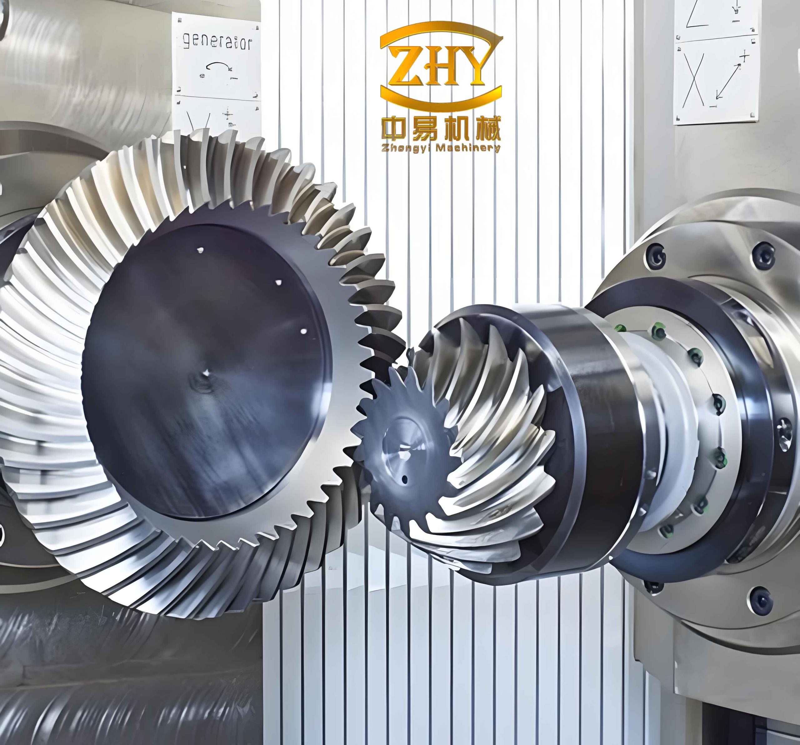
Modeling the pinion tooth surface for hyperboloidal gears is more complex due to the generating process. The cutter tilt and rotation introduce two additional rotations. The pinion cutter surface, defined by parameters \(u_p\) and \(\theta_p\), must also satisfy the equation of meshing with the imaginary generating gear (represented by the cradle). This equation states that the relative velocity between the cutter and the workpiece at the contact point must be orthogonal to the common surface normal.
$$ \mathbf{n}^{(c)} \cdot \mathbf{v}^{(cp)} = 0 $$
This condition introduces the generating roll ratio \(i_{01} = \omega_w / \omega_c\) (workpiece angular speed / cradle angular speed) and links the cradle rotation angle \(\phi_c\) (or equivalently the pinion rotation angle \(\phi_1\)) to the surface parameters. The final pinion surface is defined by a system of equations derived from the coordinate transformations and the equation of meshing:
$$ \mathbf{r}_1(u_p, \theta_p, \phi_1) = \mathbf{M}_{ps1}(i_1, j_1, S_{r1}, q_1, E_1, X_{B1}, \delta_{M1}, X_1, \phi_1) \cdot \mathbf{r}_t^{(p)}(u_p, \theta_p) $$
$$ f_{mesh}(u_p, \theta_p, \phi_1) = 0 $$
For a complete and accurate digital model of hyperboloidal gears, especially for stress analysis, the fillet (root transition) surface must be modeled. This surface is generated by the cutter tip corner with a specified radius \(r_{gf}\). Its equation is derived similarly, but the cutter surface vector \(\mathbf{r}_t^{(f)}\) is now a function of an additional parameter \(\gamma_g\) describing the arc of the tip radius.
$$ \mathbf{r}_t^{(f)}(\theta_g, \gamma_g) = \begin{bmatrix} (r_G – u_{g0}\sin\alpha_2 \pm r_{gf}\cos\alpha_2 \mp r_{gf}\sin\gamma_g) \cos\theta_g \\ (r_G – u_{g0}\sin\alpha_2 \pm r_{gf}\cos\alpha_2 \mp r_{gf}\sin\gamma_g) \sin\theta_g \\ -u_{g0}\cos\alpha_2 \mp r_{gf}\sin\alpha_2 + r_{gf}\cos\gamma_g \\ 1 \end{bmatrix} $$
The resulting discrete point clouds for the pinion and gear flanks and fillets are then interpolated to create smooth surfaces, which are used to generate a solid 3D CAD model via Boolean operations. This model serves as the basis for all subsequent analysis.
Before examining loaded behavior, unloaded Tooth Contact Analysis (TCA) is performed to assess the basic meshing quality of the hyperboloidal gears. TCA determines the path of contact and transmission error under no-load conditions by solving the conditions of continuous contact between the theoretical pinion and gear surfaces. The fundamental equations require that at the contact point, the position vectors and the surface normals (after being transformed into a fixed assembly coordinate system \(S_H\)) coincide.
$$ \mathbf{r}_1^{(H)}(\theta_p, \phi_1) = \mathbf{r}_2^{(H)}(u_g, \theta_g, \phi_2) $$
$$ \mathbf{n}_1^{(H)}(\theta_p, \phi_1) = \mathbf{n}_2^{(H)}(u_g, \theta_g, \phi_2) $$
By prescribing the pinion rotation angle \(\phi_1\), this system of vector equations can be solved numerically for the remaining five unknowns (\(\theta_p, u_g, \theta_g, \phi_2\)) and the contact point coordinates. Repeating this process for a full mesh cycle yields the transmission error (TE), defined as the deviation from perfectly conjugate motion:
$$ \delta(\phi_1) = (\phi_2 – \phi_2^0) – \frac{z_1}{z_2}(\phi_1 – \phi_1^0) $$
where \(z_1, z_2\) are the number of teeth, and \(\phi_1^0, \phi_2^0\) are initial reference angles. TCA also predicts the unloaded contact pattern (ellipse) on the tooth flank by considering the local curvature relationship between the contacting surfaces.
To analyze the real-world behavior of hyperboloidal gears, loaded tooth contact analysis (LTCA) is essential. While analytical LTCA methods exist, the Finite Element Method (FEM) provides a powerful and general approach to compute deformations, stresses, and actual contact pressure distributions under load. The accurately generated 3D CAD model is imported into a pre-processor for meshing. Due to the computational cost of modeling the full gear set, a segment model is often used: a full pinion is meshed against a sector of the gear containing several teeth (e.g., 3-5 teeth on either side of the contacting pair).
The finite element model setup involves defining material properties (typically alloy steel), applying appropriate boundary conditions, and defining the contact interaction. A key aspect is the application of load and motion. A common and efficient method is to apply a rotational speed to the pinion’s reference node (coupling all nodes on its bore) and a resisting torque to the gear’s reference node. The analysis is typically performed as a static, quasi-static, or non-linear dynamic step, accounting for large deformations and frictional contact.
| Parameter | Typical Value / Setting |
|---|---|
| Material (e.g., 20MnCr5 or similar) | Steel |
| Young’s Modulus, \(E\) | 209 GPa |
| Poisson’s Ratio, \(\nu\) | 0.3 |
| Density, \(\rho\) | 7850 kg/m³ |
| Contact Formulation | Surface-to-Surface |
| Sliding Formulation | Finite Sliding |
| Friction Coefficient, \(\mu\) | 0.05 – 0.15 (often 0.1) |
| Constraint Type | “Hard” Contact (Penalty method often used) |
| Element Type | C3D8R (8-node linear brick, reduced integration) |
| Analysis Type | Static, General (with Non-linear Geometry ON) |
From the FEM solution, critical time-varying meshing characteristics of the hyperboloidal gears can be extracted throughout the mesh cycle. The primary output is the dynamic mesh force \(F_m(t)\), which is the resultant force transmitted between the pinion and gear teeth. It exhibits periodic fluctuations at the tooth meshing frequency and its harmonics. The amplitude of these fluctuations is highly sensitive to the applied load \(T\).
$$ F_m(t) = F_{m,mean} + \sum_k A_k \sin(k\omega_m t + \psi_k) $$
where \(\omega_m\) is the meshing frequency (\(\omega_m = z_1 \cdot \Omega_1 / (2\pi)\)), and \(A_k\) are harmonic amplitudes that increase with load.
The loaded transmission error \(\delta_L(\phi_1)\) is perhaps the most critical dynamic excitation source. It is calculated from the FEM results by comparing the actual output gear rotation under load to its theoretical rigid-body position. Under load, tooth deflections (bending, shear, contact) alter the contact points and paths, significantly changing the TE function compared to its unloaded shape. The peak-to-peak value \(\Delta \delta_L\) is a key indicator of gear noise potential.
The time-varying mesh stiffness \(k_m(t)\) is a fundamental parameter for dynamic modeling. It is defined as the ratio of the dynamic mesh force to the total deflection along the line of action at any instant \(t\).
$$ k_m(t) = \frac{F_m(t)}{\delta_{def}(t)} $$
Here, \(\delta_{def}(t)\) is the composite elastic deflection of the mating tooth pairs, which can be derived from the FEM-computed rotations and the base circle radii, or directly from contact penetration data. The stiffness varies periodically because the number of tooth pairs in contact changes (from 2 to 3 for most hyperboloidal gears) and because the effective cantilever length of each tooth changes as the contact point moves across the face.
The actual contact ratio \(\varepsilon_\gamma\) under load is not a constant but an instantaneous value that can exceed the theoretical geometric contact ratio. Under heavy load, tooth deflections cause the contact to spread, potentially engaging adjacent teeth earlier and disengaging them later than predicted by rigid-body geometry. This effective contact ratio can be inferred from the mesh stiffness curve or directly from the number of tooth pairs sharing significant contact force in the FEM results at each time step.
| Meshing Parameter | Trend with Increasing Torque Load \(T\) | Primary Cause |
|---|---|---|
| Dynamic Mesh Force Fluctuation Amplitude | Increases significantly | Higher contact & bending deflections alter load sharing between tooth pairs. |
| Loaded Transmission Error (Peak-to-Peak, \(\Delta \delta_L\)) | Initially increases, may then stabilize or decrease slightly at very high load* | Deflections shift contact; optimal load may align contact pattern, reducing fluctuation. |
| Mean Mesh Stiffness | Increases | Load spreading engages more of the tooth flank and adjacent teeth more firmly. |
| Amplitude of Stiffness Variation | Increases and profile becomes asymmetric | Peak stiffness occurs earlier in mesh cycle as contact shifts toward the heel (thicker part of tooth). |
| Instantaneous Contact Ratio | Increases, especially at low-to-mid loads | Tooth deflections cause earlier engagement and later disengagement. |
| Contact Pattern Location & Size | Shifts from center towards heel and toe; expands to cover more of active flank. | Shaft wind-up and tooth bending under load. |
* The behavior of \(\Delta \delta_L\) is non-monotonic and highly dependent on initial alignment and gear geometry.
The analysis of hyperboloidal gears under varying operational conditions reveals profound insights into their dynamic behavior. A critical observation is the pronounced asymmetry that develops in the time-varying mesh stiffness curve as the load increases. Under light load, the stiffness curve is relatively symmetric, reflecting the geometric symmetry of the unloaded contact path. As torque rises, tooth and shaft deflections cause the initial contact at the start of a mesh cycle to occur closer to the gear heel (the thicker, outer part of the tooth). This region has higher local stiffness due to greater material support. Consequently, the mesh stiffness rises more sharply to an earlier peak. As the contact moves toward the toe (thinner section), the stiffness decreases, but the path is not the mirror image of the rising edge, resulting in an asymmetric waveform. This asymmetry has direct implications for the spectral content of the dynamic excitation.
Furthermore, the relationship between load and transmission error is complex. While unloaded TE is a function of manufacturing alignment and ease-off topography, loaded TE incorporates the system’s compliance. For a well-designed pair of hyperboloidal gears, there often exists an optimal load range where the loaded contact pattern best conforms to the designed ease-off, minimizing the peak-to-peak TE fluctuation. At loads below this range, the contact may not be fully established across the ideal area, leading to higher fluctuations. At excessively high loads, although the pattern expands, non-linear deflections and edge contact can again increase TE variation. Therefore, the goal in design is not necessarily to minimize TE at zero load, but to shape the ease-off so that the loaded TE is minimal and smooth across the intended operating torque spectrum.
The increase in the instantaneous contact ratio with load is another vital damping mechanism in hyperboloidal gears. At low torque, the actual number of tooth pairs carrying significant load can be close to the theoretical geometric value. As load increases, bending deflections allow the following tooth pair to come into contact before the theoretical engagement point and delay the separation of the preceding pair. This effectively increases the load-sharing capability and reduces the load per tooth pair, which in turn lowers bending stress and mitigates dynamic overloads. This phenomenon is particularly important during start-up, shock loading, or in low-torque cruising conditions where gear whine might otherwise be prominent.
The comprehensive digital modeling and analysis pipeline for hyperboloidal gears—from precise mathematical generation and TCA to detailed non-linear finite element analysis—provides an unparalleled understanding of their performance. Key findings underscore that the meshing characteristics of hyperboloidal gears are not static properties but are dynamically shaped by the operating load. Parameters like mesh stiffness, transmission error, and contact ratio exhibit significant time-varying behavior, the amplitude and pattern of which are heavily load-dependent. The emergence of asymmetric stiffness profiles under load and the non-linear relationship between load and transmission error fluctuation are critical considerations for predicting noise, vibration, and durability. These insights, derived from integrated digital tools, enable the optimization of hyperboloidal gear designs for smooth, quiet, and reliable operation across their entire operational envelope, from light cruise to peak torque conditions.