
In the field of mechanical engineering, the design and manufacturing of hyperboloidal gears have always been a challenging task due to their complex geometry and high precision requirements. Hyperboloidal gears, also known as hypoid gears, are widely used in automotive, aerospace, and heavy machinery industries because of their ability to transmit motion between non-intersecting axes with high efficiency and load capacity. Traditional methods, such as the Gleason system, involve numerous formulas and manual calculations, which are tedious and prone to errors. In this study, we propose an integrated approach using Excel, Matlab, and UG to achieve precise three-dimensional modeling of hyperboloidal gears. This method leverages the computational power of these software tools to streamline the design process, from geometric parameter calculation to solid model generation, thereby enhancing accuracy and efficiency.
The motivation behind this research stems from the growing demand for high-performance hyperboloidal gears in modern applications. For instance, in the automotive industry, the need for quieter and more durable gear systems has driven the development of advanced modeling techniques. Traditional modeling methods often rely on simulated cutting processes or machine-specific equations, which limit flexibility and require extensive knowledge of manufacturing constraints. By contrast, our approach is based on gear meshing principles, independent of specific machine tools, thus providing a foundation for subsequent special machining processes. In this article, we will detail the step-by-step methodology, including geometric design via Excel, numerical computation via Matlab, and 3D modeling via UG, along with an application example to demonstrate the effectiveness of the proposed framework.
Before delving into our method, it is essential to understand the limitations of conventional hyperboloidal gear modeling techniques. Typically, these methods can be categorized into two types: one involves computer simulation of cutting processes, such as the HFT tool tilt method, to generate the gear tooth surface, followed by entity modeling using CAD software; the other derives the tooth surface equation based on cutter dimensions and motion analysis, which is then solved and fitted into a model. Both approaches are constrained by machine tool and cutter specifications, making them less adaptable to design variations. Moreover, the calculation process is cumbersome, requiring manual adjustments and verification. Therefore, there is a clear need for a more automated and accurate modeling strategy, which we address by combining spreadsheet calculations, mathematical programming, and advanced CAD capabilities.
Our proposed methodology for precise modeling of hyperboloidal gears integrates three software platforms: Excel for geometric parameter design, Matlab for numerical computation and discrete point generation, and UG for 3D solid modeling. Each tool plays a critical role in the pipeline, as summarized in the following table:
| Software | Primary Function | Key Features Utilized |
|---|---|---|
| Excel | Geometric parameter calculation and design | Formula automation, error analysis, data tabulation |
| Matlab | Numerical solution of tooth profile equations | Matrix operations, function plotting, discrete point extraction |
| UG | 3D solid modeling and surface fitting | Curve fitting, scanning, Boolean operations, array functions |
The general process begins with inputting initial gear parameters into an Excel spreadsheet, which automatically computes key geometric values. These values are then used to derive mathematical models of the tooth profile, which are solved numerically in Matlab to generate discrete coordinate points. Finally, the points are imported into UG to create curves and surfaces, leading to a complete 3D model of the hyperboloidal gear. This approach not only reduces human error but also significantly speeds up the design cycle, making it suitable for iterative optimization and custom gear designs.
Let us first explore the role of Excel in the design of hyperboloidal gears. Excel is a widely used spreadsheet program that offers powerful functions for data management and calculation. In our context, we developed a customized Excel template that incorporates all necessary formulas for hyperboloidal gear geometry, based on established gear theory. The template allows users to input basic parameters, such as tooth numbers, gear width, and offset distance, and then automatically computes derived parameters like pitch angles, cone distances, and backlash. This automation is achieved through built-in mathematical and trigonometric functions, as well as logical operations for error checking. For example, the following table illustrates a subset of parameters calculated for a typical hyperboloidal gear design:
| Parameter | Symbol | Value (Example) | Formula/Note |
|---|---|---|---|
| Number of teeth (pinion) | z1 | 10 | Input |
| Number of teeth (gear) | z2 | 41 | Input |
| Gear width | b2 | 30 mm | Input |
| Offset distance | E | 20 mm | Input |
| Pitch angle (pinion) | δ1 | 15.5° | Calculated from gear ratio |
| Cone distance | R | 125.4 mm | $$ R = \frac{0.5 m z}{\sin \delta} $$ |
| Base cone angle | β | 12.3° | Derived from mesh conditions |
By using Excel, we can quickly iterate through different design scenarios, ensuring that the hyperboloidal gears meet specific performance criteria. The spreadsheet also facilitates documentation and sharing of design data, which is crucial for collaborative engineering projects. Once the geometric parameters are finalized, we proceed to the mathematical modeling of the tooth profile, which is implemented in Matlab.
Matlab is a high-level programming environment renowned for its numerical computation capabilities. In our study, we use Matlab to solve the tooth profile equations derived from gear meshing theory. The end-face tooth profile of a hyperboloidal gear consists of four segments: the tip arc, the spherical involute, the root fillet, and the root arc. Each segment is governed by a parametric equation, which we analyze and discretize to obtain coordinate points. The key equations are as follows:
1. Spherical Involute Equation: This represents the main tooth flank, derived from the geometry of a sphere. The parametric form is:
$$ x = R(\sin \phi \sin \theta + \cos \phi \cos \theta \sin \psi) $$
$$ y = R(\cos \phi \sin \theta \sin \psi – \sin \phi \cos \theta) $$
$$ z = R \cos \phi \cos \psi $$
where \( R \) is the cone distance, \( \phi = \theta \sin \beta \) is the angle between a radial line and the instantaneous axis, \( \theta \) is the parameter along the involute, \( \beta \) is the base cone angle, and \( \psi \) is the rotation angle about the axis. These equations describe the complex curvature of hyperboloidal gears, essential for accurate meshing.
2. Tip Arc Equation: This corresponds to the top land of the tooth:
$$ x = R \sin \alpha_t \cos \varphi_t $$
$$ y = R \sin \alpha_t \sin \varphi_t $$
$$ z = R \cos \alpha_t $$
where \( \alpha_t \) is the tip cone angle (the angle between the radial vector and the z-axis), and \( \varphi_t \) is the azimuthal angle in the XY-plane. This arc is trimmed with other segments to form the tooth tip.
3. Root Arc Equation: This forms the bottom land:
$$ x = R \sin \alpha_r \cos \varphi_r $$
$$ y = R \sin \alpha_r \sin \varphi_r $$
$$ z = R \cos \alpha_r $$
where \( \alpha_r \) is the root cone angle, and \( \varphi_r \) is the corresponding azimuthal angle.
4. Tooth Length Line Equation: This defines the path along the tooth face:
$$ x = R \sin \alpha_f \cos \varphi_f $$
$$ y = R \sin \alpha_f \sin \varphi_f $$
$$ z = R \cos \alpha_f $$
where \( \alpha_f \) is the face cone angle, and \( \varphi_f \) varies along the tooth length.
In Matlab, we write scripts to compute these equations over specified parameter ranges. For instance, for the spherical involute, we discretize \( \theta \) from 0 to a maximum value based on tooth geometry, and for each \( \theta \), calculate \( x, y, z \) coordinates. The output is a matrix of discrete points, which we save as a text file. Matlab’s plotting functions allow us to visualize the curves, but for precise modeling, we export the raw data for use in UG. The following pseudo-code illustrates the Matlab process for the spherical involute:
% Parameters
R = 125.4; % cone distance (mm)
beta = 12.3 * pi/180; % base cone angle (rad)
theta_range = linspace(0, 0.5, 100); % parameter range
psi = 0; % fixed for end-face section

% Initialize arrays
x_points = [];
y_points = [];
z_points = [];

for theta = theta_range
    phi = theta * sin(beta);
    x = R * (sin(phi)*sin(theta) + cos(phi)*cos(theta)*sin(psi));
    y = R * (cos(phi)*sin(theta)*sin(psi) - sin(phi)*cos(theta));
    z = R * cos(phi) * cos(psi);
    x_points = [x_points; x];
    y_points = [y_points; y];
    z_points = [z_points; z];
end

% Save to file
data = [x_points, y_points, z_points];
save('involute_points.txt', 'data', '-ascii');
By running similar scripts for all tooth profile segments, we generate multiple point clouds that collectively define the tooth geometry. These point clouds are then imported into UG for surface reconstruction and solid modeling.
UG (now part of Siemens NX) is a advanced CAD/CAM/CAE software with robust surface and solid modeling tools. In our workflow, we use UG to create the 3D entity of the hyperboloidal gear based on the discrete points from Matlab. The process involves several steps: first, we import the point data files into UG, typically by converting them to a .doc format that UG can read directly. Then, we use the curve fitting function to generate smooth curves from the points. For example, the points from the spherical involute equation are fitted into a spline curve representing the tooth flank. Similarly, points from the tip and root arcs are used to create circular arcs. These curves are then combined to form a closed loop for the end-face tooth profile.
Next, we create the tooth length line by fitting points from the tooth length equation. This line serves as a guide for sweeping the end-face profile along the tooth direction. Using UG’s sweep function, we generate a solid tooth by sweeping the profile along the path. This results in a single tooth entity with accurate geometry. To complete the hyperboloidal gear, we first create a gear blank based on the back cone parameters calculated in Excel. The blank is a conical solid representing the gear body. Then, we use Boolean operations to subtract the tooth cavity from the blank, and finally, array the tooth around the axis to form the full gear set. The following table summarizes the UG modeling steps:
| Step | Action in UG | Details |
|---|---|---|
| 1 | Import point data | Load .doc files containing coordinates from Matlab |
| 2 | Fit curves | Use spline fitting to create curves from points |
| 3 | Create end-face profile | Combine curves into a closed loop |
| 4 | Generate tooth length path | Fit a curve along tooth direction |
| 5 | Sweep profile | Sweep end-face profile along path to form solid tooth |
| 6 | Create gear blank | Model conical blank using back cone parameters |
| 7 | Boolean subtraction | Subtract tooth from blank to create cavity |
| 8 | Array teeth | Circular array to replicate tooth around gear |
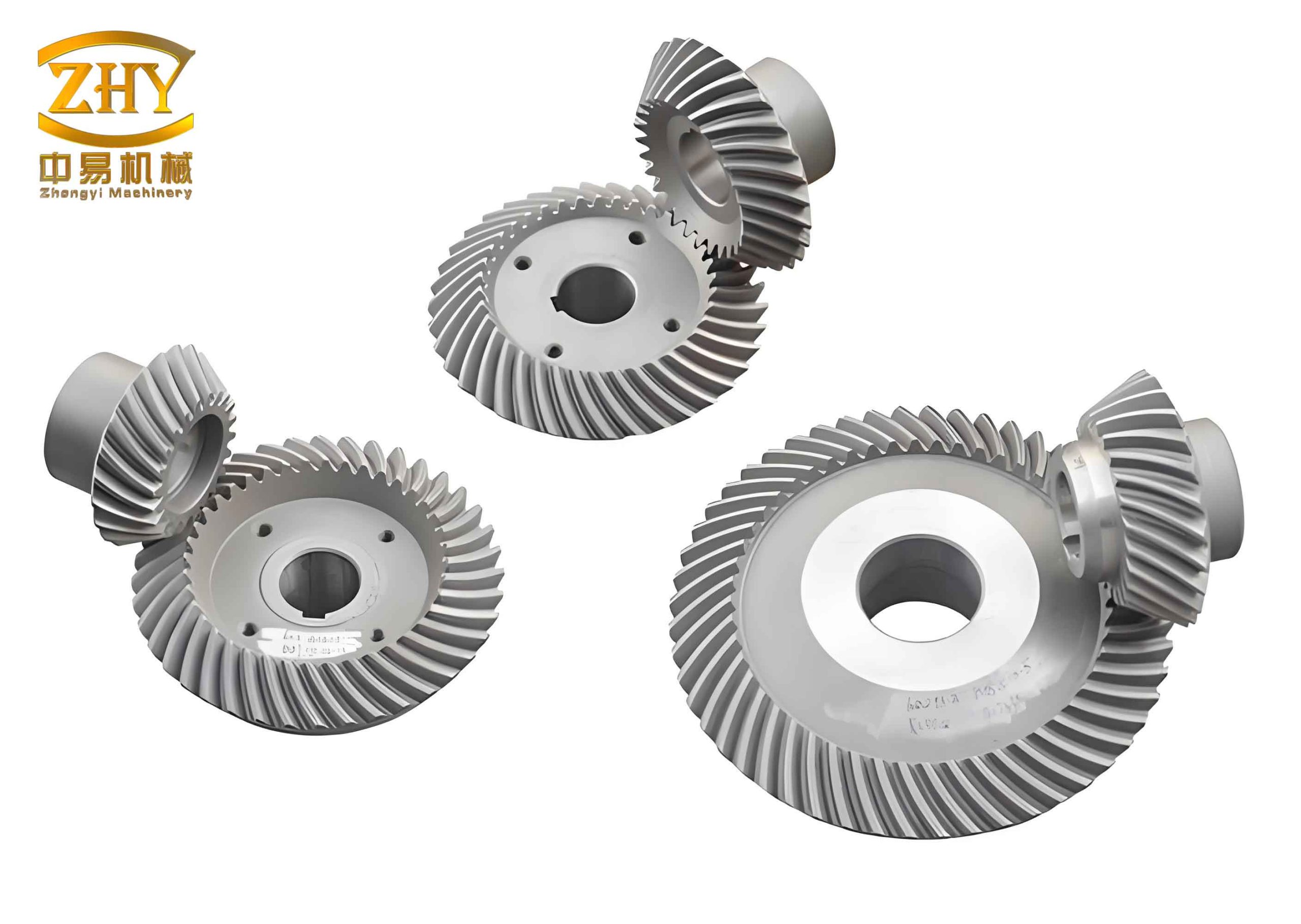
To illustrate the modeling outcome, we include a visual representation of a hyperboloidal gear generated through this process. The image below shows the intricate geometry of these gears, highlighting the curved teeth and offset axes characteristic of hyperboloidal gears.
Now, let us walk through a detailed application example to demonstrate the entire methodology. Suppose we are designing hyperboloidal gears for an automotive rear axle, with the following initial parameters: pinion teeth \( z1 = 10 \), gear teeth \( z2 = 41 \), gear width \( b2 = 30 \) mm, and offset distance \( E = 20 \) mm. We start by entering these values into our Excel spreadsheet, which computes all necessary geometric parameters. The spreadsheet includes formulas for cone distance, pitch angles, and backlash, among others. For instance, the cone distance \( R \) is calculated using:
$$ R = \frac{0.5 m z}{\sin \delta} $$
where \( m \) is the module, and \( \delta \) is the pitch angle. The module is derived from the gear ratio and size constraints. After computation, we obtain key values such as \( R = 125.4 \) mm, base cone angle \( \beta = 12.3^\circ \), and tip cone angle \( \alpha_t = 18.7^\circ \). These are used in the subsequent Matlab and UG stages.
In Matlab, we implement the tooth profile equations with the computed parameters. For the spherical involute, we set \( R = 125.4 \), \( \beta = 12.3^\circ \), and discretize \( \theta \) from 0 to 0.5 radians with 200 points to ensure smoothness. The script generates coordinate points for the involute, as well as for the tip arc, root arc, and tooth length line. Each point set is saved in separate text files. We also validate the curves by plotting them in Matlab, as shown in the figure below (note: the figure is not included here, but in practice, it helps verify accuracy).
Next, we import the point files into UG. Using the curve fitting tool, we create splines for each segment. For example, the involute points form a curved line that matches the theoretical tooth flank. We then trim and join the curves to create a closed profile for the end-face. Simultaneously, we fit the tooth length points into a path curve that runs along the gear’s conical surface. With both profile and path ready, we perform a sweep operation to generate a solid tooth. This tooth is then positioned on the gear blank, which we modeled earlier as a cone with dimensions from Excel. Through Boolean subtraction, we cut the tooth space into the blank, and finally, use circular patterning to create all teeth. The result is a precise 3D model of the hyperboloidal gear, ready for simulation or manufacturing.
The advantages of this integrated approach are manifold. First, by using Excel, we automate the complex calculations involved in hyperboloidal gear design, reducing human error and saving time. The spreadsheet can be easily modified for different gear specifications, making it a versatile tool. Second, Matlab’s numerical capabilities allow us to handle intricate equations efficiently, producing accurate discrete points for CAD modeling. This is crucial for hyperboloidal gears, where tooth geometry directly impacts performance. Third, UG’s advanced modeling functions enable us to convert mathematical data into a tangible 3D entity, which can be used for finite element analysis, assembly checks, or CNC programming. Together, these tools form a seamless pipeline that enhances the design and development of hyperboloidal gears.
In conclusion, our study presents a robust methodology for precise modeling of hyperboloidal gears using Excel, Matlab, and UG. This approach addresses the limitations of traditional methods by leveraging software automation and numerical computation. We have demonstrated through an application example that the method yields accurate 3D models suitable for engineering applications. Future work could focus on integrating this pipeline with optimization algorithms to further improve gear performance, or extending it to other types of gears. The use of hyperboloidal gears is expected to grow in advanced mechanical systems, and our methodology provides a foundation for efficient and accurate design processes. By combining calculation, computation, and modeling, we pave the way for innovation in gear technology.
To further elaborate on the mathematical foundations, let us discuss the derivation of the spherical involute equation in more detail. The spherical involute is generated by a point on a great circle of a sphere as it rolls without slipping on a base circle. This concept is analogous to planar involutes but extended to spherical geometry. The parametric equations can be derived using vector analysis and spherical trigonometry. Consider a sphere of radius \( R \), with a base cone of angle \( \beta \). The position vector of a point on the involute can be expressed as:
$$ \mathbf{r} = R \left( \sin \phi \sin \theta \, \mathbf{i} + (\cos \phi \sin \theta \sin \psi – \sin \phi \cos \theta) \, \mathbf{j} + \cos \phi \cos \psi \, \mathbf{k} \right) $$
where \( \mathbf{i}, \mathbf{j}, \mathbf{k} \) are unit vectors along the coordinate axes. This formulation ensures that the tooth profile satisfies the meshing conditions for hyperboloidal gears. The complexity of these equations underscores the need for numerical tools like Matlab.
In terms of implementation, we have developed a comprehensive Excel template that includes error-checking mechanisms. For instance, if the calculated pressure angle exceeds recommended limits, the template flags a warning, prompting the designer to adjust input parameters. This proactive approach minimizes design flaws early in the process. Additionally, the template outputs a summary table, as shown below, which serves as a reference for all subsequent steps:
| Design Parameter | Value | Unit | Status |
|---|---|---|---|
| Pinion teeth (z1) | 10 | – | Input |
| Gear teeth (z2) | 41 | – | Input |
| Offset distance (E) | 20 | mm | Input |
| Module (m) | 4.5 | mm | Calculated |
| Cone distance (R) | 125.4 | mm | Calculated |
| Base cone angle (β) | 12.3 | ° | Calculated |
| Tip cone angle (α_t) | 18.7 | ° | Calculated |
| Root cone angle (α_r) | 10.2 | ° | Calculated |
| Pressure angle | 20 | ° | Checked |
Moving to Matlab, we emphasize the importance of discretization accuracy. The number of points generated for each curve affects the smoothness of the final UG model. Through trial and error, we determined that 200 points per curve segment provide a good balance between detail and file size. Matlab scripts also include visualization codes to plot the points in 3D, allowing us to inspect the tooth profile before exporting. For example, we can use the `plot3` function to display the spherical involute and ensure it matches theoretical expectations. This step is crucial for validating the input parameters and equations.
In UG, the curve fitting process uses non-uniform rational B-splines (NURBS) to approximate the discrete points. UG’s algorithms ensure that the fitted curves are smooth and continuous, which is essential for generating high-quality surfaces. After sweeping the profile along the path, we obtain a solid tooth that can be analyzed for geometric properties, such as volume and center of mass. UG also allows us to perform draft analysis to ensure manufacturability, though that is beyond the scope of this study. The final gear model can be exported in standard formats like STEP or IGES for use in other software.
One of the key benefits of this methodology is its adaptability to different types of hyperboloidal gears. Whether for automotive differentials or industrial machinery, the same pipeline can be applied with minor adjustments. Moreover, the use of hyperboloidal gears in high-torque applications necessitates precise modeling to avoid stress concentrations and noise. Our approach facilitates this by providing a digital twin of the gear, which can be used in finite element analysis (FEA) to predict performance under load. For instance, the 3D model from UG can be imported into FEA software like ANSYS to simulate contact stresses and tooth deflection.
In summary, the integration of Excel, Matlab, and UG offers a comprehensive solution for the precise modeling of hyperboloidal gears. This method not only improves accuracy and efficiency but also enables advanced analyses that are critical for modern engineering. As technology advances, such integrated approaches will become increasingly important in the design and manufacturing of complex mechanical components. We hope that this research contributes to the ongoing development of gear technology and inspires further innovations in the field.