
The advancement of robotics and mechatronics has imposed stringent requirements on gear transmissions, particularly demanding high reduction ratios. Hyperboloidal gears, evolved from hypoid gears, represent a conical worm-wheel type transmission that retains all the advantages of hypoid gears while achieving significant speed reduction and enabling motion transfer between non-parallel, non-intersecting axes. While international companies like GLEASON have established design and manufacturing theories for high-reduction hyperboloidal gears, technological barriers have limited domestic research, which has primarily focused on machining and fundamental design theories. Due to their exceptionally high transmission ratios, wear in these gears is a critical issue, often leading to the premature failure of the pinion before the gear reaches its service life. Therefore, studying wear mechanisms and optimization strategies for high-reduction hyperboloidal gears is of considerable significance.
In common gear wear research, many studies focus on tribological properties, calculating wear amounts based on various wear theories to assess wear conditions. However, establishing accurate wear prediction models that match real-world conditions presents significant challenges and limitations. Beyond wear volume, the sliding rate between gear teeth is closely related to surface wear. The sliding rate can reflect the transmission performance of a gear pair to some extent. Theoretical and experimental results show that a larger absolute value of the sliding rate indicates more severe relative sliding between tooth flanks, increasing the risk of surface scuffing. To improve the wear and scuffing resistance of high-reduction hyperboloidal gears, analyzing the causes of sliding and studying the sliding rate can provide a foundation for wear optimization.
This paper first introduces a novel method for calculating the tooth blank parameters of high-reduction hyperboloidal gears, deriving formulas for basic dimensions. Subsequently, based on spatial gear meshing principles, the kinematic state of point-contact gear pairs is analyzed to derive the fundamental sliding rate equation. Combining this with the basic transmission principles of high-reduction hyperboloidal gears, the motion state at the pitch point is analyzed, leading to the derivation of a sliding rate formula expressed as a function of the gear blank design parameters.
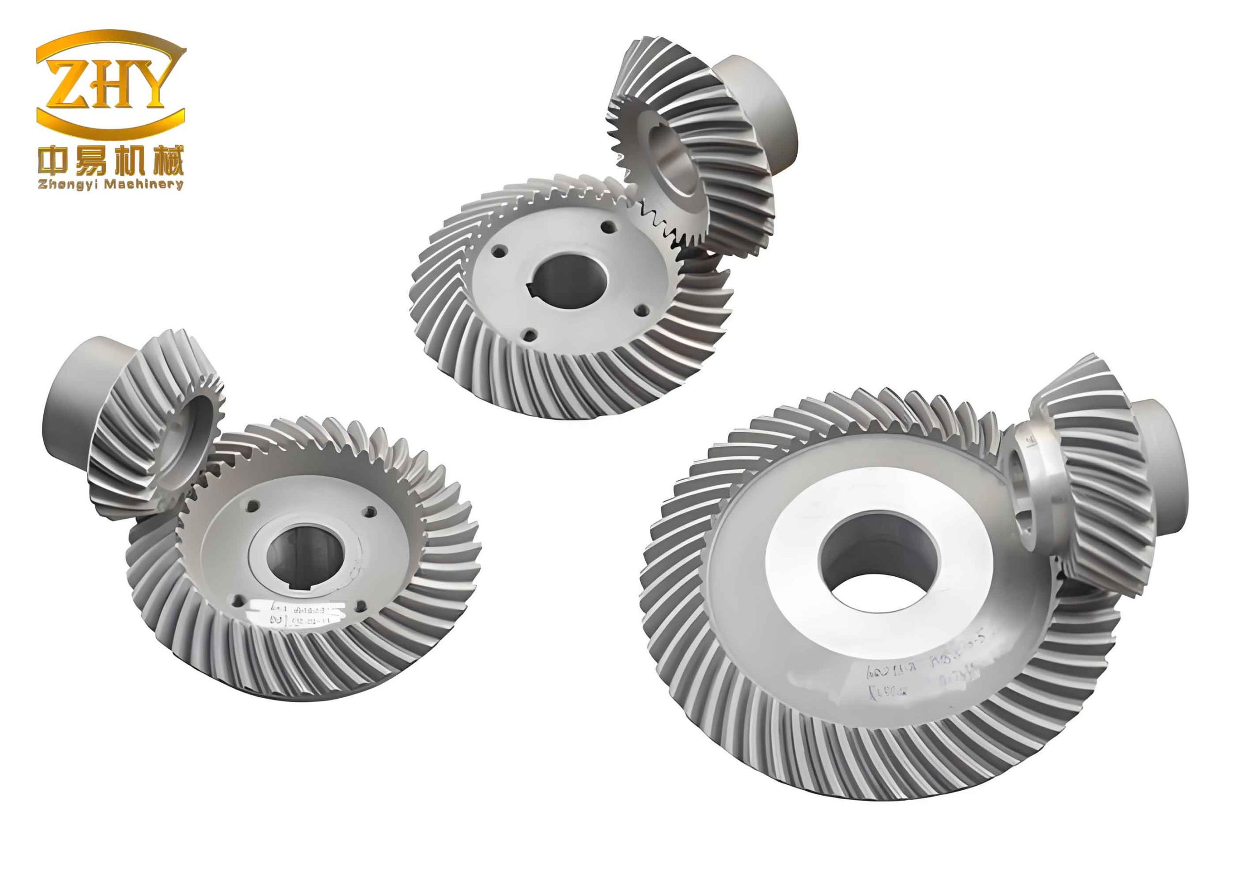
Tooth Blank Parameter Calculation for High-Reduction Hyperboloidal Gears
Derived from hypoid gears, high-reduction hyperboloidal gears maintain the advantages of their predecessors while breaking the tooth number limitations of conventional hypoid gears and improving transmission efficiency. This section proposes a calculation method for determining the pinion blank parameters of high-reduction gears starting from the gear parameters, referencing the GLEASON hypoid gear blank calculation methodology. The determination of the spatial pitch point position is key to defining the pitch cones of a hyperboloidal gear pair. From geometry, defining a point in space requires three independent parameters. The pitch point location is determined using the gear pitch radius \(r_2\), the pinion spiral angle \(\beta_1\), and the pinion axial section offset angle \(\eta\). The following discusses the method for determining these three parameters and derives the basic blank dimensions for both gear and pinion.
First, based on transmission requirements, the shaft angle \(\Sigma\), number of teeth for gear and pinion \(Z_2, Z_1\), hand of spiral, and pinion offset distance \(E\) are determined. The gear pitch diameter \(d_2\) can be selected based on load capacity requirements. The selected gear face width \(b_2\) should not exceed \(10 \times m_t\) (where \(m_t = d_2 / Z_2\)) or one-third of the outer cone distance of a spiral bevel gear under similar conditions. An approximate formula recommended by GLEASON is used to determine the gear pitch angle:
$$ \tan \delta_2′ = \frac{\sin \Sigma}{1.2(z_2 / z_1 + \cos \Sigma)} $$
After the gear pitch cone is determined, the gear pitch radius is calculated as:
$$ r_2 = \frac{1}{2}(d_2 – b_2 \sin \delta_2′) $$
The gear axial section offset angle is determined by:
$$ \sin \epsilon_0′ = \frac{E \sin \delta_2′}{r_2} $$
\(\beta_{20}\) is the initial given value for the pinion spiral angle, typically \(\beta_{20} \approx 35^\circ\). An initial pinion enlargement factor \(k’\) is introduced:
$$ k’ = \frac{1}{\cos \epsilon_0′ – \tan \beta_{20} \sin \epsilon_0′} $$
The initial pinion pitch radius is:
$$ r_1′ = k’ i_{12} r_2 $$
where \(i_{12}\) is the gear ratio, \(i_{12} = Z_1 / Z_2\). The pinion axial section offset angle is obtained iteratively:
$$ \tan \eta_1′ = \frac{r_2 \tan \delta_2′}{E – (r_2 \tan \delta_2′ \sin \Sigma)/\tan \Sigma + r_1′} $$
If \(|\tan \eta_1’| \le 0.01\), set \(\tan \eta_1′ = \pm 0.011\), with the sign matching that of the calculated value. Depending on whether \(\tan \eta_1′ < 0\) or \(> 0\), approximate values for the gear axial section offset angle \(\epsilon\), pinion pitch angle \(\delta_1\), offset angle \(\epsilon’\), and pinion spiral angle \(\beta_1\) are calculated:
$$
\begin{aligned}
\sin \epsilon &= (E – r_1′ \sin \eta_1′) / r_2 \\
\tan \delta_1′ &= \tan \eta_1′ / \sin \Sigma – \cot \Sigma \cos \eta_1′ \\
\sin \epsilon’ &= \tan \eta_1′ \sin \Sigma / \sin \delta_1′ \\
\cos \beta_1′ &= \cos \epsilon’ / \sqrt{1 – \sin^2 \epsilon’ \sin^2 \delta_1′}
\end{aligned}
$$
The approximate gear spiral angle is found by:
$$ \sin \beta_2′ = \frac{\cos \epsilon_1′ – 1/k’}{\sin \epsilon_1′} $$
The value \(\beta_2’\) obtained from Eq. (8) may not equal the desired spiral angle \(\beta_{20}\). The enlargement factor is then corrected to adjust the pinion pitch radius. The corrected factor is \(k = 1/(\cos \epsilon_1′ – \tan \beta_{20} \sin \epsilon_1′)\). Subtracting this from \(k_1′ = 1/(\cos \epsilon_1′ – \tan \beta_2′ \sin \epsilon_1′)\) yields a new enlargement factor, and a new pinion pitch radius \(r_1 = k i_{12} r_2\) is calculated.
Recalculate the values for \(\epsilon, \delta_1, \epsilon’, \beta_1\):
$$
\begin{aligned}
\sin \epsilon &= \sin \epsilon_1′ – i_{12}(k – k’) \sin \eta_1′ / k \\
\tan \delta_1 &= \tan \eta_1′ / \sin \Sigma – \cot \Sigma \cos \eta_1′ \\
\tan \epsilon’ &= (\cos \epsilon – 1/k) / \sin \epsilon \\
\beta_1 &= \beta_1′ + \arcsin(\sin \epsilon’ \sin \delta_1′)
\end{aligned}
$$
The gear pitch angle is given by:
$$ \tan \delta_2 = \frac{\sin \epsilon}{\tan \eta_1′ \sin \Sigma} – \cot \Sigma \cos \epsilon $$
Then the gear pitch cone distance is \(R_2 = r_2 / \sin \delta_2\). The pinion pitch cone distance is:
$$ R_1 = \frac{r_1 + i_{12}(k – k’) r_2}{\sin \delta_1} $$
Thus, the pinion pitch radius is \(r_1 = R_1 \sin \delta_1\). The limiting pressure angle \(\alpha^*\) is calculated as:
$$ \tan \alpha^* = \frac{R_1 \tan \delta_1 – R_2 \tan \delta_2}{\cos \epsilon (\tan \delta_1 + \tan \delta_2) – (R_1 \tan \beta_1 + R_2 \tan \beta_2)} $$
The limiting curvature radius is found by:
$$ \frac{1}{r^*} = \frac{ \frac{\tan \beta_1}{R_1 \cos \delta_1} – \frac{\tan \beta_2}{R_2 \cos \delta_2} }{ \tan \alpha^* (\frac{1}{R_1 \tan \delta_1} + \frac{1}{R_2 \tan \delta_2}) + (\frac{1}{R_1 \cos \beta_1} + \frac{1}{R_2 \cos \beta_2}) } $$
If \(|1 – r_0 / r^*| < 0.01\), the iteration ends, where \(r_0\) is the nominal cutter radius. If \(|1 – r_0 / r^*| \ge 0.01\), the first trial fails. Set \(\tan \eta_2 = \tan \eta_1′ – 0.01\) and iterate again. For the second iteration, \(\tan \eta_3 = \tan \eta_2 – 0.01[1 – (r_0/r^*)_2^2] / [(r_0/r^*)_2^2 – (r_0/r^*)_1^2]\). Iteration continues until the condition is satisfied.
Through the above derivation and iterative calculation, the fundamental blank parameters for the high-reduction hyperboloidal gears are obtained. The design of these hyperboloidal gears relies heavily on precise geometric definitions to ensure proper meshing under high reduction ratios.
Kinematic Analysis of Spatial Meshing
To understand the sliding mechanisms in hyperboloidal gears, a general analysis of spatial gear meshing is necessary. Three coordinate systems are established in space: \(S\), \(S_1\), and \(S_2\). System \(S\) is the fixed coordinate system with origin \(O\). Systems \(S_1\) and \(S_2\) are attached to gear 1 and gear 2, respectively, with origins \(O_1\) and \(O_2\) located on their axes. The angular velocities of the two gears are \(\boldsymbol{\omega}^{(1)}\) and \(\boldsymbol{\omega}^{(2)}\). The translational velocities of \(S_1\) and \(S_2\) in space are \(\boldsymbol{v}_0^{(1)}\) and \(\boldsymbol{v}_0^{(2)}\).
Selecting a point \(M\) in space, the vectors \(\overrightarrow{O_1M} = \boldsymbol{r}^{(1)}\) and \(\overrightarrow{O_2M} = \boldsymbol{r}^{(2)}\). The vectors \(\overrightarrow{OO_1} = \boldsymbol{r}_0^{(1)}\) and \(\overrightarrow{OO_2} = \boldsymbol{r}_0^{(2)}\). When point \(M\) moves with \(S_1\), its velocities in the \(S\) coordinate are \(\boldsymbol{v}^{(1)}\) and \(\boldsymbol{v}^{(2)}\), respectively. The relative velocity of gear 1 with respect to gear 2 at point \(M\) is \(\boldsymbol{v}^{(12)}\). For point \(M\):
$$ \boldsymbol{r} = \boldsymbol{r}_0^{(1)} + \boldsymbol{r}^{(1)} $$
Differentiating with respect to time \(t\) and transforming according to the relationship between vector increments in moving and fixed frames yields:
$$ \frac{d\boldsymbol{r}}{dt} = \boldsymbol{\omega}^{(1)} \times \boldsymbol{r}^{(1)} + \frac{d_1 \boldsymbol{r}^{(1)}}{dt} + \boldsymbol{v}_0^{(1)} $$
Similarly, starting from \(\boldsymbol{r} = \boldsymbol{r}_0^{(2)} + \boldsymbol{r}^{(2)}\), after transformation we obtain:
$$ d_2 \boldsymbol{r}^{(2)} = d_1 \boldsymbol{r}^{(1)} + \boldsymbol{v}^{(12)} dt $$
This equation shows that the motion of point \(M\) along the two tooth surfaces generally has different directions. If the direction of \(d_1 \boldsymbol{r}^{(1)}\) is chosen to be that of \(\boldsymbol{v}^{(12)}\), then \(d_2 \boldsymbol{r}^{(2)}\) also aligns with \(\boldsymbol{v}^{(12)}\). However, they differ by \(\boldsymbol{v}^{(12)} dt\), meaning there is relative sliding with velocity \(\boldsymbol{v}^{(12)}\) during meshing. This is the fundamental cause of sliding in gear tooth engagement.
The sliding ratios \(\sigma_1\) and \(\sigma_2\) on the tooth surfaces can be expressed in terms of the relative differentials of point \(M\) along the surfaces:
$$
\begin{aligned}
\sigma_1 &= \frac{|d_1 \boldsymbol{r}^{(1)}| – |d_2 \boldsymbol{r}^{(2)}|}{|d_1 \boldsymbol{r}^{(1)}|} \\
\sigma_2 &= \frac{|d_2 \boldsymbol{r}^{(2)}| – |d_1 \boldsymbol{r}^{(1)}|}{|d_2 \boldsymbol{r}^{(2)}|}
\end{aligned}
$$
According to established gear meshing theory, the sliding rate between tooth surfaces can be calculated by the formula:
$$
\begin{aligned}
\sigma_1 &= \frac{(\boldsymbol{v}^{(12)}, \boldsymbol{\omega}^{(12)}, \boldsymbol{n}) + |\boldsymbol{v}^{(12)}| (k_v^{(1)} \boldsymbol{n} \cdot \boldsymbol{q})}{(\boldsymbol{v}^{(12)}, \boldsymbol{\omega}^{(12)}, \boldsymbol{n}) + |\boldsymbol{v}^{(12)}| (k_v^{(2)} \boldsymbol{n} \cdot \boldsymbol{q})} – 1 \\
\sigma_2 &= \frac{(\boldsymbol{v}^{(12)}, \boldsymbol{\omega}^{(12)}, \boldsymbol{n}) + |\boldsymbol{v}^{(12)}| (k_v^{(2)} \boldsymbol{n} \cdot \boldsymbol{q})}{(\boldsymbol{v}^{(12)}, \boldsymbol{\omega}^{(12)}, \boldsymbol{n}) + |\boldsymbol{v}^{(12)}| (k_v^{(1)} \boldsymbol{n} \cdot \boldsymbol{q})} – 1
\end{aligned}
$$
where \(\boldsymbol{q} = (\boldsymbol{\omega}^{(1)} \times (\boldsymbol{\omega}^{(2)} \times \boldsymbol{r}^{(2)}) – \boldsymbol{\omega}^{(2)} \times (\boldsymbol{\omega}^{(1)} \times \boldsymbol{r}^{(1)}))\), \(\boldsymbol{n}\) is the unit normal vector to the tooth surface, and \(k_v^{(1)}, k_v^{(2)}\) are the normal curvatures of the surfaces in the direction of relative velocity.
Sliding Rate Derivation for High-Reduction Hyperboloidal Gears
Based on the tooth blank parameters for high-reduction hyperboloidal gears derived in Section 1, the pitch point \(M\) on both gears is determined. According to the spatial geometric relationship during meshing of hyperboloidal gears, a coordinate system \((M-\boldsymbol{i}, \boldsymbol{j}, \boldsymbol{k})\) with its origin at the pitch point is established. The angular velocity vectors \(\boldsymbol{\omega}^{(1)}\) and \(\boldsymbol{\omega}^{(2)}\) lie along the gear axes. Vectors \(\boldsymbol{i}\) and \(\boldsymbol{j}\) lie in the pitch plane, and \(\boldsymbol{k}\) is perpendicular to it. The pitch plane is tangent to the two pitch cones along lines \(O’M\) and \(O”M\) with lengths \(L_1\) and \(L_2\), respectively.
When \(M\) rotates about axes \(O’B’\) and \(O”B”\), the relative velocity \(\boldsymbol{v}^{(12)}\) lies in the pitch plane. We have:
$$
\begin{aligned}
\overrightarrow{O’M} &= L_1 (-\sin\beta_1 \boldsymbol{i} – \cos\beta_1 \boldsymbol{j}) \\
\overrightarrow{O”M} &= L_2 (-\sin\beta_2 \boldsymbol{i} – \cos\beta_2 \boldsymbol{j})
\end{aligned}
$$
The angular velocities can be expressed as:
$$
\begin{aligned}
\boldsymbol{\omega}^{(1)} &= \omega_1 (-\cos\delta_1 \sin\beta_1 \boldsymbol{i} – \cos\delta_1 \cos\beta_1 \boldsymbol{j} + \sin\delta_1 \boldsymbol{k}) \\
\boldsymbol{\omega}^{(2)} &= \omega_2 (\cos\delta_2 \sin\beta_2 \boldsymbol{i} + \cos\delta_2 \cos\beta_2 \boldsymbol{j} – \sin\delta_2 \boldsymbol{k})
\end{aligned}
$$
The relative angular velocity is:
$$
\begin{aligned}
\boldsymbol{\omega}^{(12)} &= (\omega_1 \cos\delta_1 \sin\beta_1 + \omega_2 \cos\delta_2 \sin\beta_2) \boldsymbol{i} \\
&+ (\omega_1 \cos\delta_1 \cos\beta_1 + \omega_2 \cos\delta_2 \cos\beta_2) \boldsymbol{j} \\
&+ (-\omega_1 \sin\delta_1 – \omega_2 \sin\delta_2) \boldsymbol{k}
\end{aligned}
$$
From the above, the velocity vectors are:
$$
\begin{aligned}
\boldsymbol{v}^{(1)} &= \boldsymbol{\omega}^{(1)} \times \overrightarrow{O’M} = \omega_1 L_1 (\sin\delta_1 \sin\beta_1 \boldsymbol{i} + \sin\delta_1 \cos\beta_1 \boldsymbol{j}) \\
\boldsymbol{v}^{(2)} &= \boldsymbol{\omega}^{(2)} \times \overrightarrow{O”M} = \omega_2 L_2 (\sin\delta_2 \sin\beta_2 \boldsymbol{i} + \sin\delta_2 \cos\beta_2 \boldsymbol{j})
\end{aligned}
$$
Choosing \(\boldsymbol{v}^{(12)}\) to be parallel to the \(\boldsymbol{j}\)-axis (so its \(\boldsymbol{i}\)-component is zero), the relative velocity simplifies to:
$$ \boldsymbol{v}^{(12)} = (\omega_1 L_1 \sin\delta_1 \sin\beta_1 – \omega_2 L_2 \sin\delta_2 \sin\beta_2) \boldsymbol{j} $$
Using the functional relationships between the gear blank parameters, this can be transformed into:
$$ |\boldsymbol{v}^{(12)}| = \omega_1 L_1 \sin\delta_1 \frac{\sin \epsilon’}{\cos \beta_2} $$
The characteristic vector \(\boldsymbol{q}\) expressed in design parameters is:
$$
\begin{aligned}
\boldsymbol{q} &= \omega_1 \omega_2 [ L_1 \sin\delta_1 \sin\delta_2 (\sin\beta_2 – \sin\beta_1) \boldsymbol{i} \\
&- (L_1^2 \sin\delta_1 \sin\delta_2 (\cos\beta_1 + \cos\beta_2) + L_1 L_2 \cos\epsilon’ (\sin\delta_1 \cos\delta_2 + \cos\delta_1 \sin\delta_2)) \boldsymbol{j} \\
&+ L_2 \cos\epsilon’ (L_1 \sin\delta_1 \cos\delta_2 + L_2 \cos\delta_1 \sin\delta_2) \boldsymbol{k} ]
\end{aligned}
$$
The unit normal vector to the tooth surface is \(\boldsymbol{n} = \pm \cos\alpha \boldsymbol{i} + \sin\alpha \boldsymbol{k}\), where \(\alpha\) is the pressure angle. The upper sign (+) applies to the gear concave side (pinion convex side), and the lower sign (-) applies to the opposite. The limiting pressure angle \(\alpha_0\) at the boundary point of meshing is:
$$ \tan \alpha_0 = \pm \frac{L_1 \sin\beta_1 – L_2 \sin\beta_2}{L_1 \tan\delta_1 + L_2 \tan\delta_2} $$
The limiting normal vector is \(\boldsymbol{n}_0 = \pm \cos\alpha_0 \boldsymbol{i} + \sin\alpha_0 \boldsymbol{k}\). After transformation:
$$ \boldsymbol{n} \cdot \boldsymbol{k} = \frac{\sin(\alpha – \alpha_0)}{\cos\alpha_0} $$
From the analysis, \(\boldsymbol{n} \cdot \boldsymbol{q}\) and the scalar triple product \((\boldsymbol{v}^{(12)}, \boldsymbol{\omega}^{(12)}, \boldsymbol{n})\) can be calculated:
$$ \boldsymbol{n} \cdot \boldsymbol{q} = \omega_1 \omega_2 \frac{\sin(\alpha – \alpha_0)}{\cos\alpha_0} [ L_2 \cos\epsilon’ (L_1 \sin\delta_1 \cos\delta_2 + L_2 \cos\delta_1 \sin\delta_2) ] $$
And,
$$
\begin{aligned}
(\boldsymbol{v}^{(12)}, \boldsymbol{\omega}^{(12)}, \boldsymbol{n}) &= \begin{vmatrix}
0 & \omega_1 L_1 \sin\delta_1 \sin\beta_1 – \omega_2 L_2 \sin\delta_2 \sin\beta_2 & 0 \\
\omega_1 \cos\delta_1 \sin\beta_1 + \omega_2 \cos\delta_2 \sin\beta_2 & \omega_1 \cos\delta_1 \cos\beta_1 + \omega_2 \cos\delta_2 \cos\beta_2 & -\omega_1 \sin\delta_1 – \omega_2 \sin\delta_2 \\
\pm\cos\alpha & 0 & \sin\alpha
\end{vmatrix} \\
&= [\omega_1 L_1 \sin\delta_1 \sin\beta_1 – \omega_2 L_2 \sin\delta_2 \sin\beta_2] \cdot \\
&\quad [(\omega_1 \cos\delta_1 \sin\beta_1 + \omega_2 \cos\delta_2 \sin\beta_2)(\sin\alpha) – (-\omega_1 \sin\delta_1 – \omega_2 \sin\delta_2)(\pm\cos\alpha)]
\end{aligned}
$$
Substituting equations (23), (27), and (28) into the general sliding rate formula (17) yields the sliding rate formula for high-reduction hyperboloidal gears as a function of their design parameters. For the gear surface (considered as surface 1), the sliding rate \(\sigma_1\) is:
$$
\sigma_1 = \frac{ \begin{vmatrix} 0 & V_{12y} & 0 \\ \omega_{12x} & \omega_{12y} & \omega_{12z} \\ \pm\cos\alpha & 0 & \sin\alpha \end{vmatrix} + |\boldsymbol{v}^{(12)}| (k_v^{(1)} \cdot N_q ) }{ \begin{vmatrix} 0 & V_{12y} & 0 \\ \omega_{12x} & \omega_{12y} & \omega_{12z} \\ \pm\cos\alpha & 0 & \sin\alpha \end{vmatrix} + |\boldsymbol{v}^{(12)}| (k_v^{(2)} \cdot N_q ) } – 1
$$
where:
$$ V_{12y} = \omega_1 L_1 \sin\delta_1 \sin\beta_1 – \omega_2 L_2 \sin\delta_2 \sin\beta_2 = \omega_1 L_1 \sin\delta_1 \frac{\sin \epsilon’}{\cos \beta_2} $$
$$ \omega_{12x} = \omega_1 \cos\delta_1 \sin\beta_1 + \omega_2 \cos\delta_2 \sin\beta_2 $$
$$ \omega_{12y} = \omega_1 \cos\delta_1 \cos\beta_1 + \omega_2 \cos\delta_2 \cos\beta_2 $$
$$ \omega_{12z} = -\omega_1 \sin\delta_1 – \omega_2 \sin\delta_2 $$
$$ N_q = \omega_1 \omega_2 \frac{\sin(\alpha – \alpha_0)}{\cos\alpha_0} [ L_2 \cos\epsilon’ (L_1 \sin\delta_1 \cos\delta_2 + L_2 \cos\delta_1 \sin\delta_2) ] $$
The normal curvature \(k_v^{(1)}\) for the gear tooth surface can be calculated using relevant formulas from spiral bevel gear theory. The formula for the pinion sliding rate \(\sigma_2\) is analogous but lengthy and is omitted here for brevity. This derived formula establishes a direct relationship between the fundamental design parameters of high-reduction hyperboloidal gears and the sliding rate at their pitch point, providing a valuable tool for wear analysis.
Sliding Rate Calculation and Verification for Gear Examples
Using the tooth blank calculation method proposed in the first section, the basic design parameters for two sets of high-reduction hyperboloidal gears with ratios of 5:60 and 3:45 were calculated, as shown in Tables 1 and 2 below. These parameters are crucial for the subsequent sliding rate analysis of these hyperboloidal gears.
| Component | Pinion | Gear |
|---|---|---|
| Number of Teeth, z | 3 | 45 |
| Normal Module, m_n (mm) | 1.067 | |
| Offset Distance, E (mm) | 10 | |
| Pressure Angle, α (°) | 20 | |
| Shaft Angle, Σ (°) | 90 | |
| Face Width, b (mm) | 9.24 | 5.76 |
| Spiral Angle, β (°) | 67.10 | 39.00 |
| Pitch Angle, δ (°) | 10.99 | 77.60 |
| Outer Diameter (mm) | 10.41 | 48.01 |
| Component | Gear | Pinion |
|---|---|---|
| Number of Teeth, z | 60 | 5 |
| Normal Module, m_n (mm) | 1.360 | |
| Offset Distance, E (mm) | 14 | |
| Pressure Angle, α (°) | 19 | |
| Shaft Angle, Σ (°) | 90 | |
| Face Width, b (mm) | 16.08 | 13.50 |
| Spiral Angle, β (°) | 55.15 | 31.12 |
| Pitch Angle, δ (°) | 5.33 | 84.17 |
| Outer Diameter (mm) | 14.10 | 81.65 |
Taking the gear concave side (pinion convex side) as the study object, and considering the gear tooth surface as the first surface, the parameters from the two gear sets were substituted into the derived sliding rate formula. The results are shown in Table 3.
| Gear Set | |σ₁| (Gear) | |σ₂| (Pinion) |
|---|---|---|
| 3:45 | 1.2381 | 5.1999 |
| 5:60 | 0.6364 | 1.7505 |
The calculated values show that the absolute sliding rate for the gear is smaller than that for the pinion. This result aligns with the practical observation that wear conditions on the gear are generally better than on the pinion during meshing of hyperboloidal gears. To further verify the validity of the formula, a spatial coordinate system was established based on the spatial position relationship between the pitch cones of the high-reduction gears. Using the parameters of the 5:60 gear set, the spatial coordinates of the pitch point were determined. These coordinates and related data were substituted into the algebraic expression for sliding rate found in the literature and solved using MATLAB, yielding \(|\sigma_1’| = 0.6176\) and \(|\sigma_2’| = 1.7613\). This verification result also shows that the absolute sliding rate value for the gear is smaller than that for the pinion, following the same trend, which further confirms the correctness of the derived sliding rate calculation formula for hyperboloidal gears.
Conclusion
Through the study on the calculation method for the sliding rate of high-reduction hyperboloidal gears, the following conclusions are drawn:
-
A novel iterative calculation method for determining the basic tooth blank parameters of high-reduction hyperboloidal gears, starting from the gear parameters, was proposed. This method provides a new design approach for the blank design of high-reduction hyperboloidal gears, which is essential for their manufacture and performance.
-
Based on the spatial gear sliding rate calculation formula, the sliding rate formula at the pitch point for high-reduction hyperboloidal gears was derived. This establishes a correlation model between the design parameters and the pitch point sliding rate, providing a theoretical foundation for wear optimization studies of high-reduction hyperboloidal gears.
-
Two gear pairs with tooth number ratios of 3:45 and 5:60 were studied as examples. The calculated absolute values of the sliding rate at the tooth surface pitch point were 1.2381 and 0.6364 for the gears, and 5.1999 and 1.7505 for the pinions, respectively. The results indicate that the sliding rate at the pitch point of meshing high-reduction hyperboloidal gears is not zero; relative sliding exists at the pitch point. This inherent sliding contributes to the wear characteristics of these hyperboloidal gear transmissions and must be considered in their design for longevity and reliability.
The research on hyperboloidal gears, especially those with high reduction ratios, is critical for advancing power transmission in compact and demanding applications like robotics. Understanding and quantifying parameters like the sliding rate is a key step towards improving the durability and efficiency of these complex mechanical components.