
1. Introduction
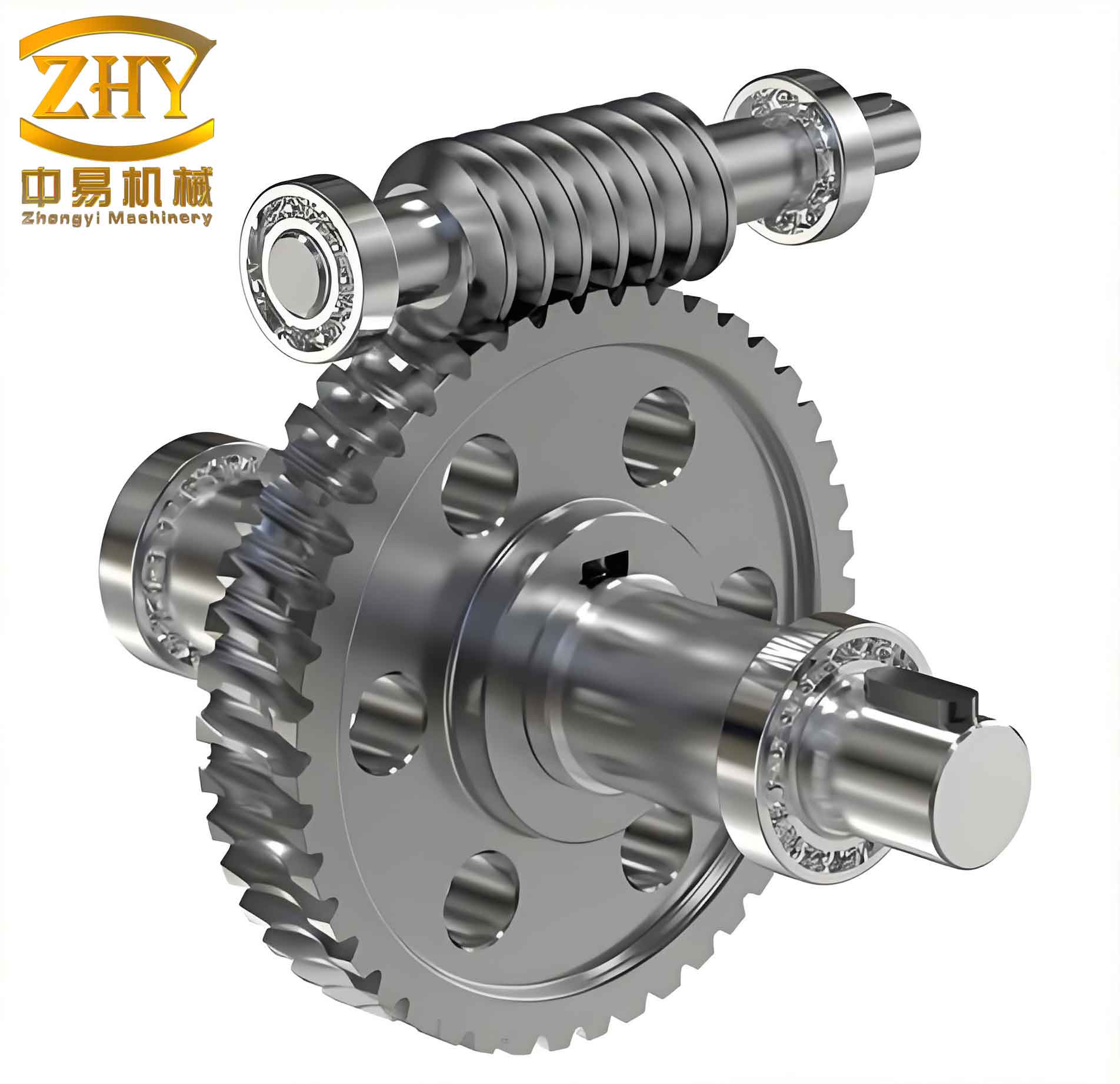
Worm gears constitute a critical branch of gear transmission, operating on inclined plane principles that differ fundamentally from the lever-based mechanics typical of standard gear pairs. A defining characteristic of worm gear systems is the substantial relative sliding velocity between conjugate tooth flanks, which inevitably accelerates surface wear. Converting this sliding friction into rolling friction represents a highly effective strategy for reducing the friction coefficient and enhancing transmission efficiency. Various innovative designs have been proposed in the literature to achieve this objective. For instance, Kato and colleagues introduced pin-wheel worm gearing and conducted comprehensive investigations into its structural design, manufacturing processes, efficiency, and lubrication conditions. The SANKYO Corporation successfully commercialized roller enveloping hourglass worm gears for reducer applications. Similarly, Siegmund and others developed ball-based hourglass worm drives, incorporating steel balls as worm wheel teeth and employing small steel spheres within ball sockets to minimize sliding friction between the balls and the wheel body.
Significant theoretical and experimental progress has been made in related domains. Zhang and Chen, among others, proposed and systematically studied rolling cone enveloping hourglass worm drives, covering meshing theory, parameter optimization, prototype manufacturing, and performance testing. Their work confirmed that such systems offer high efficiency, substantial load capacity, extended service life, and simplified manufacturing. Deng and colleagues introduced backlash-free double-roller enveloping hourglass worm drives, where the worm is generated by enveloping the worm wheel tooth surface, and each wheel tooth consists of two rollers capable of rotation about their own axes. This design not only retains the advantages of high efficiency, multiple meshing teeth, and strong load capacity but also provides adjustability for backlash, enabling zero-backlash operation. Further studies have addressed meshing geometry for spherical enveloping hourglass worm gears, the influence of errors on contact patterns, time-varying mesh stiffness, and lubrication flow field analysis. Despite this extensive research, most prior work has focused on theoretical performance, design optimization, or lubrication under ideal conditions, often neglecting the practical impact of assembly errors. Pure theoretical models do not adequately reflect real-world contact scenarios, and the absence of quantitative guidance on how assembly errors affect tooth surface contact can lead to issues like poor meshing or even seizure during operation.
To bridge this gap, we develop an interference analysis model for roller enveloping hourglass worm gear pairs that explicitly accounts for assembly errors. We propose quantitative evaluation metrics for interference and systematic computational methods. We then analyze the influence of four specific errors: center distance deviation, worm axial displacement, worm wheel axial displacement, and shaft intersection angle error, on the contact behavior of the transmission pair.
2. Basic Meshing Geometry of Roller Enveloping Hourglass Worm Gears
2.1 Coordinate Systems and Transformations
In a roller enveloping hourglass worm drive, the worm wheel is an assembly featuring cylindrical rollers as its teeth. The hourglass worm tooth surface is generated by enveloping the roller cylindrical surface according to prescribed conjugate motion. To describe this relationship, we establish a set of coordinate systems. Two fixed reference frames, σm (om–xmymzm) and σn (on–xnynzn), define the initial positions of the worm wheel and worm, respectively. A moving frame σ1 (o1–x1y1z1) is rigidly attached to the worm wheel, rotating about the z1-axis with angular velocity ω1. Similarly, a moving frame σ2 (o2–x2y2z2) is attached to the hourglass worm, rotating about the z2-axis with angular velocity ω2. The instantaneous angular displacements are φ1 and φ2, related by the transmission ratio i12 = ω1/ω2 = φ1/φ2 = Z2/Z1, where Z1 is the number of worm threads and Z2 is the number of worm wheel teeth. The center distance is denoted by a.
The transformation from the worm wheel frame σ1 to the worm frame σ2 is given by:
$$ (x_2, y_2, z_2, 1)^T = M_{n2} M_{mn} M_{1m} (x_1, y_1, z_1, 1)^T $$
where the transformation matrices are defined as:
$$ M_{1m} = \begin{bmatrix} \cos\phi_1 & -\sin\phi_1 & 0 & 0 \\ \sin\phi_1 & \cos\phi_1 & 0 & 0 \\ 0 & 0 & 1 & 0 \\ 0 & 0 & 0 & 1 \end{bmatrix} $$
$$ M_{mn} = \begin{bmatrix} -1 & 0 & 0 & a \\ 0 & 0 & 0 & 0 \\ 0 & 1 & 1 & 0 \\ 0 & 0 & 0 & 1 \end{bmatrix} $$
$$ M_{n2} = \begin{bmatrix} \cos\phi_2 & -\sin\phi_2 & 0 & 0 \\ \sin\phi_2 & \cos\phi_2 & 0 & 0 \\ 0 & 0 & 1 & 0 \\ 0 & 0 & 0 & 1 \end{bmatrix} $$
2.2 Roller Tooth Surface
In the worm wheel fixed coordinate system σ1, the position vector of a point on the cylindrical roller tooth surface is expressed using surface parameters u (along the roller axis) and θ (angular parameter). The roller radius is r.
The position vector r1 is given by:
$$ \mathbf{r}_1 = x_1\mathbf{i}_1 + y_1\mathbf{j}_1 + z_1\mathbf{k}_1 $$
$$ \begin{cases} x_1 = u \\ y_1 = -r \sin\theta \\ z_1 = r \cos\theta \end{cases} $$
The unit normal vector n1 to the roller surface in this frame is:
$$ \mathbf{n}_1 = n_{x1}\mathbf{i}_1 + n_{y1}\mathbf{j}_1 + n_{z1}\mathbf{k}_1 $$
$$ \begin{cases} n_{x1} = 0 \\ n_{y1} = -\sin\theta \\ n_{z1} = \cos\theta \end{cases} $$
2.3 Meshing Equation
For continuous meshing between the hourglass worm and the roller tooth surfaces, they must remain in tangency at all contact points. This condition is expressed by the fundamental equation of meshing:
$$ \Phi = \mathbf{v}^{(12)} \cdot \mathbf{n}_1 = 0 $$
where v(12) is the relative velocity vector at the point of contact. To simplify computation without loss of generality, we set ω2 = 1 rad/s, giving ω1 = i12 rad/s. The components of the relative velocity in the σ1 frame are:
$$ \mathbf{v}^{(12)} = v^{(12)}_{1x}\mathbf{i}_1 + v^{(12)}_{1y}\mathbf{j}_1 + v^{(12)}_{1z}\mathbf{k}_1 $$
$$ \begin{cases} v^{(12)}_{1x} = z_1 \cos\phi_1 – i_{12} y_1 \\ v^{(12)}_{1y} = i_{12} x_1 – y_1 \sin\phi_1 \\ v^{(12)}_{1z} = -x_1 \cos\phi_1 + y_1 \sin\phi_1 + a \end{cases} $$
Substituting the expressions for v(12) and n1 into the meshing condition yields the meshing function for roller enveloping hourglass worm gears:
$$ \Phi(u, \theta, \phi_1) = a i_{12} \cos\theta – u \sin\theta – u i_{12} \cos\phi_1 \cos\theta = 0 $$
2.4 Contact Lines on the Roller Surface
The instantaneous contact lines on the roller tooth surface are defined by the set of points that simultaneously satisfy the roller surface equation and the meshing equation.
The contact line equation is:
$$ \begin{cases} \mathbf{r}_1(u, \theta) = x_1\mathbf{i}_1 + y_1\mathbf{j}_1 + z_1\mathbf{k}_1 \\ \Phi(u, \theta, \phi_1) = 0 \end{cases} $$
2.5 Hourglass Worm Tooth Surface
The theoretical hourglass worm tooth surface is obtained by transforming the contact lines from the roller surface into the worm fixed coordinate system σ2.
The worm tooth surface equation is:
$$ \begin{cases} \mathbf{r}_2(u, \theta, \phi_1) = x_2\mathbf{i}_2 + y_2\mathbf{j}_2 + z_2\mathbf{k}_2 \\ \Phi(u, \theta, \phi_1) = 0 \end{cases} $$
The components of the position vector in the σ2 frame are:
$$ \begin{aligned} x_2 &= a\cos\phi_2 – u\cos\phi_1\cos\phi_2 – r\cos\theta\sin\phi_2 – r\cos\phi_2\sin\phi_1\sin\theta \\ y_2 &= a\sin\phi_2 + r\cos\theta\cos\phi_2 – u\cos\phi_1\sin\phi_2 – r\sin\phi_1\sin\phi_2\sin\theta \\ z_2 &= u\sin\phi_1 – r\cos\phi_2\sin\theta \end{aligned} $$
3. Mathematical Model of the Transmission Pair with Assembly Errors
3.1 Coordinate Systems and Transformations with Errors
During actual assembly, it is practically impossible to achieve perfect positioning, and various errors inevitably arise. We decompose these assembly errors into their directional components and consider four specific types: center distance error, worm axial error, worm wheel axial error, and shaft intersection angle error. For analytical convenience and without loss of generality, we assume the worm wheel is mounted in its ideal, error-free position. Consequently, all errors are attributed to the relative displacement of the hourglass worm with respect to the worm wheel.
The transformation matrix between the worm fixed frame σm and the worm wheel fixed frame σn must be modified to incorporate these errors:
$$ M_{mn} = \begin{bmatrix} -1 & 0 & 0 & a + \Delta a \\ 0 & \sin\Delta\Sigma & \cos\Delta\Sigma & -\Delta L_2 \\ 0 & \cos\Delta\Sigma & -\sin\Delta\Sigma & \Delta L_1 \\ 0 & 0 & 0 & 1 \end{bmatrix} $$
where:
- Δa represents the center distance error.
- ΔL2 represents the worm axial error (axial displacement of the worm).
- ΔL1 represents the worm wheel axial error (axial displacement of the worm wheel).
- ΔΣ represents the shaft intersection angle error.
The transformations between the moving frames (σ1 to σm, and σn to σ2) remain unchanged, as displacement between the moving and fixed frames for each component is not affected by the assembly errors.
| Error Symbol | Error Name | Description |
|---|---|---|
| Δa | Center Distance Error | Deviation from the nominal center distance a |
| ΔL2 | Worm Axial Error | Axial displacement of the worm along its rotation axis |
| ΔL1 | Worm Wheel Axial Error | Axial displacement of the worm wheel along its rotation axis |
| ΔΣ | Shaft Intersection Angle Error | Angular deviation from the nominal 90° shaft angle |
3.2 Tooth Surface Equation with Errors
Under the assumption that the worm wheel is in its standard position, its tooth surface remains as defined by the error-free equation. The hourglass worm tooth surface, however, is now generated using the transformation matrix that includes the assembly errors. The resulting tooth surface equation is:
$$ \begin{cases} \mathbf{r}’_2(u, \theta, \phi_1) = x’_2\mathbf{i}_2 + y’_2\mathbf{j}_2 + z’_2\mathbf{k}_2 \\ \Phi(u, \theta, \phi_1) = 0 \end{cases} $$
The components of the position vector for the worm tooth surface with errors are:
$$
\begin{aligned}
x’_2 &= y_1 (\sin\phi_2 \cos\phi_1 – \sin\phi_1 \cos\phi_2 \sin\Delta\Sigma) \\
&\quad – x_1 (\cos\phi_1 \cos\phi_2 + \sin\phi_1 \sin\phi_2 \sin\Delta\Sigma) \\
&\quad + (a + \Delta a)\cos\phi_1 + \sin\phi_1 (\Delta L_1 \cos\Delta\Sigma – \Delta L_2 \sin\Delta\Sigma) \\
&\quad – z_1 \cos\Delta\Sigma \sin\phi_1
\end{aligned}
$$
$$
\begin{aligned}
y’_2 &= y_1 (\sin\phi_1 \sin\phi_2 + \cos\phi_1 \cos\phi_2 \sin\Delta\Sigma) \\
&\quad – x_1 (\cos\phi_2 \sin\phi_1 – \cos\phi_1 \sin\phi_2 \sin\Delta\Sigma) \\
&\quad + (a + \Delta a)\sin\phi_1 – \cos\phi_1 (\Delta L_1 \cos\Delta\Sigma – \Delta L_2 \sin\Delta\Sigma) \\
&\quad + z_1 \cos\Delta\Sigma \cos\phi_1
\end{aligned}
$$
$$
\begin{aligned}
z’_2 &= \Delta L_2 \cos\Delta\Sigma + \Delta L_1 \sin\Delta\Sigma \\
&\quad – z_1 \sin\Delta\Sigma + y_1 \cos\phi_2 \cos\Delta\Sigma \\
&\quad + x_1 \cos\Delta\Sigma \sin\phi_2
\end{aligned}
$$
3.3 Quantitative Evaluation of Interference
When assembly errors are present, the theoretically line contact between the roller and the worm tooth surface becomes an interference condition. The severity of this interference can be quantified by the cross-sectional area of the interference volume on the roller surface. Given the complex geometry, the interference cross-section often takes the form of an arbitrary curved shape. For practical computation, we approximate this cross-section as either a triangle or a quadrilateral, which significantly reduces computational effort while preserving the essential trend of the interference behavior.
Two typical forms of interference cross-sections are considered:
- Triangular Interference: The cross-section is approximated by a triangle with vertices at (xT1, yT1, zT1), (xT2, yT2, zT2), and (xT3, yT3, zT3). The interference area Si is calculated using Heron’s formula:
$$ S_i = S_{\Delta 123} = \sqrt{P(P – a_T)(P – b_T)(P – c_T)} $$
where:
$$
\begin{aligned}
a_T &= \sqrt{(x_{T1} – x_{T2})^2 + (y_{T1} – y_{T2})^2 + (z_{T1} – z_{T2})^2} \\
b_T &= \sqrt{(x_{T1} – x_{T3})^2 + (y_{T1} – y_{T3})^2 + (z_{T1} – z_{T3})^2} \\
c_T &= \sqrt{(x_{T1} – x_{T3})^2 + (y_{T1} – y_{T3})^2 + (z_{T1} – z_{T3})^2} \\
P &= (a_T + b_T + c_T) / 2
\end{aligned}
$$
- Quadrilateral Interference: The cross-section is approximated by a quadrilateral with vertices (xQ1, yQ1, zQ1), (xQ2, yQ2, zQ2), (xQ3, yQ3, zQ3), and (xQ4, yQ4, zQ4). The total area is the sum of two triangles formed by dividing the quadrilateral along a diagonal:
$$ S_i = S_{\Delta 123} + S_{\Delta 134} $$
where the area of each triangle is computed using Heron’s formula with the appropriate side lengths.
3.4 Solving for Interference Points
To calculate the interference area, the coordinates of the vertices must be determined. Consider a point j on the roller axis of the worm wheel, with coordinates (xj, yj, zj), and a point k on the hourglass worm tooth surface at the same arc height, with coordinates (xk, yk, zk). Interference occurs when the distance between these points is less than the roller radius r:
$$ \sqrt{(x_j – x_k)^2 + (y_j – y_k)^2 + (z_j – z_k)^2} < r $$
Conversely, if no contact occurs, the distance is greater than r. The vertices of the interference cross-section are located where the distance exactly equals r:
$$ \sqrt{(x_j – x_k)^2 + (y_j – y_k)^2 + (z_j – z_k)^2} = r $$
By combining the roller tooth surface equation, the worm tooth surface equation with errors, and this boundary condition, we can solve for the vertex coordinates. The solution involves discretizing the worm meshing angle φ1 over its operating range and iteratively searching for the boundary points. This process is implemented in a numerical program to compute the interference areas.
4. Case Study and Analysis of Contact Characteristics
4.1 Basic Parameters of the Example
To validate the theoretical models and analyze contact characteristics, we use a specific roller enveloping hourglass worm gear pair with the parameters listed in Table 2.
| Parameter | Symbol | Value | Unit |
|---|---|---|---|
| Center Distance | a | 80 | mm |
| Transmission Ratio | i12 | 20 | – |
| Roller Radius | r | 7 | mm |
| Roller axial parameter range | u | [56, 68] | mm |
| Worm wheel rotation angle range | φ1 | [-40, 40] | degrees |
4.2 Theoretical Contact Characteristics
Using the theoretical contact line equation, we compute and visualize the contact pattern on the roller tooth surface. The analysis reveals that the theoretical contact lines for roller enveloping hourglass worm gears are spatial helicoidal curves located in the vicinity of the mid-plane of the roller. This result confirms the fundamental meshing geometry of this transmission type.
4.3 Contact Characteristics with Assembly Errors
We systematically investigate the influence of each assembly error component on the interference area. For the analysis, we consider the sum of interference areas on both the left and right tooth flanks for selected teeth. Due to symmetry, we focus on the outer tooth 1, outer tooth 2, and the central tooth on one side.
4.3.1 Influence of Center Distance Error
The center distance error is varied within the range Δa ∈ [-0.10, 0.10] mm. The relationship between the error and the total interference area is examined.
The results indicate that different teeth exhibit varying sensitivity to the center distance error. The central tooth theoretically has zero interference area under ideal conditions, but the interference area for the outer teeth increases as the absolute value of the error increases. The rate of increase in interference area diminishes with larger errors. The outer lateral teeth display larger interference areas than the inner lateral teeth. The interference area is symmetrically distributed with respect to zero error. A positive error causes interference on the right tooth flank of the roller, while a negative error causes interference on the left flank.
4.3.2 Influence of Worm Axial Error
We analyze the worm axial error ΔL2 over the range [0.00, 0.10] mm. The worm’s axial displacement has a nearly uniform influence on all tooth pairs. The overall trend shows an increase in interference area with increasing displacement, but the rate of growth gradually slows down.
4.3.3 Influence of Worm Wheel Axial Error
The worm wheel axial error ΔL1 was also studied in the range [0.00, 0.10] mm. The influence of this error on the interference is significantly less than that of the center distance error or the worm axial error. This is because the degree of meshing engagement is minimal in the direction along the worm wheel axis. The effect on all tooth pairs is similar, with the interference area increasing slowly as the error grows.
4.3.4 Influence of Shaft Intersection Angle Error
The shaft intersection angle error ΔΣ is considered within the range [-0.5°, 0.5°], where a positive value indicates rotation in the clockwise direction. For errors within this range, the interference area for each tooth pair is relatively small. The interference area is symmetrically distributed with respect to the sign of the error. As the absolute value of the error increases, the interference area increases. The rate of change for this error is more pronounced compared to the three previous types of errors, indicating high sensitivity to angular misalignment.
The following table summarizes the sensitivity of the interference area to different error types, comparing the interference at a specific non-zero error value (e.g., 0.05 mm or 0.25 degrees). Due to the different units, the shaft intersection angle error is not directly compared in the same table with the linear errors.
| Error Type | Interference Area at Error = 0 mm (mm2) | Interference Area at Error = 0.05 mm (mm2) | Rate of Increase (approx.) |
|---|---|---|---|
| Worm Axial Error ΔL2 | 0.00 | ~1.25 | High |
| Center Distance Error Δa | 0.00 | ~0.82 | Medium |
| Worm Wheel Axial Error ΔL1 | 0.00 | ~0.35 | Low |
Table 3 provides a clear quantitative comparison. For the same magnitude of error, the worm axial error generates the largest interference area, followed by the center distance error, while the worm wheel axial error has the smallest impact.
5. Conclusion
This study has established a comprehensive interference analysis model for roller enveloping hourglass worm gear pairs, explicitly incorporating the effects of four principal assembly errors. The model enables the calculation of theoretical interference cross-sectional areas, providing a quantitative tool for evaluating the impact of manufacturing and assembly inaccuracies. Our theoretical analysis demonstrates that the ideal contact lines on the roller surface for this type of worm gear are spatial helicoidal curves located near the mid-plane of the roller.
Through systematic parametric analysis of a case study, we have quantified the influence of each error component. The results clearly show that the worm axial displacement error exerts the most significant influence on the interference area. The center distance error has a secondary level of influence, while the worm wheel axial error has the least impact. The shaft intersection angle error, despite being an angular parameter, is found to have a substantial and sensitive effect on the interference of the outer teeth, and it must be strictly controlled.
These findings offer valuable guidance for the practical manufacturing and assembly of roller enveloping hourglass worm gear systems. To ensure optimal contact conditions and minimize performance issues like excessive wear or jamming, tolerances for the worm axial displacement should be the most stringent. The shaft intersection angle should also be carefully managed. The quantitative relationships derived in this work can serve as a foundation for developing tolerance specifications and improving the overall reliability and efficiency of this advanced class of worm gears. Furthermore, the methodology developed here can be extended to analyze the influence of other error types or combined error conditions in the future. It is also crucial for the design of high-performance reducers employing these specialized worm gears. The insights gained are directly applicable to the field of precision transmission where such high-reliability worm gears are increasingly desired. The robust performance of well-assembled roller enveloping hourglass worm gears makes them a competitive choice for demanding applications.