
In this work, we propose a quasi dual-lead worm gear transmission method based on the principle of dual-lead line-contact offset worm gear transmission, and present a detailed analysis of its engineering approximate errors. By employing standard module gear hobs to cut the worm wheel and traditional Archimedes worm cutting techniques to machine the worm, we achieve a simplified manufacturing process while retaining the advantages of dual-lead offset worm gear drives. We investigate the tooth flank error sources between the quasi dual-lead worm gear transmission and the ideal dual-lead line-contact offset worm gear transmission, establish error calculation formulas, and propose measures to reduce or eliminate these errors. Two quasi dual-lead worm gear pairs with transmission ratios of 70 and 410 are designed and tested, verifying the correctness and effectiveness of the proposed method.
The concept of conical worm gear transmission was first introduced by the United States in the 1950s. It offers advantages such as large transmission ratio, smooth operation, multiple meshing teeth, high load capacity, and the possibility of using hardened steel for the conical worm wheel. The dual-lead line-contact offset worm gear transmission is a new type of conical worm gear drive that combines all the benefits of traditional conical worm gears, with simpler transmission principles and more convenient manufacturing. However, because it requires specialized cutting tools, producing single or small batches becomes costly and inconvenient. To address this issue, we propose a quasi dual-lead worm gear transmission method based on engineering approximation principles, and discuss its approximate error characteristics.
Quasi Dual-lead Worm Gear Transmission
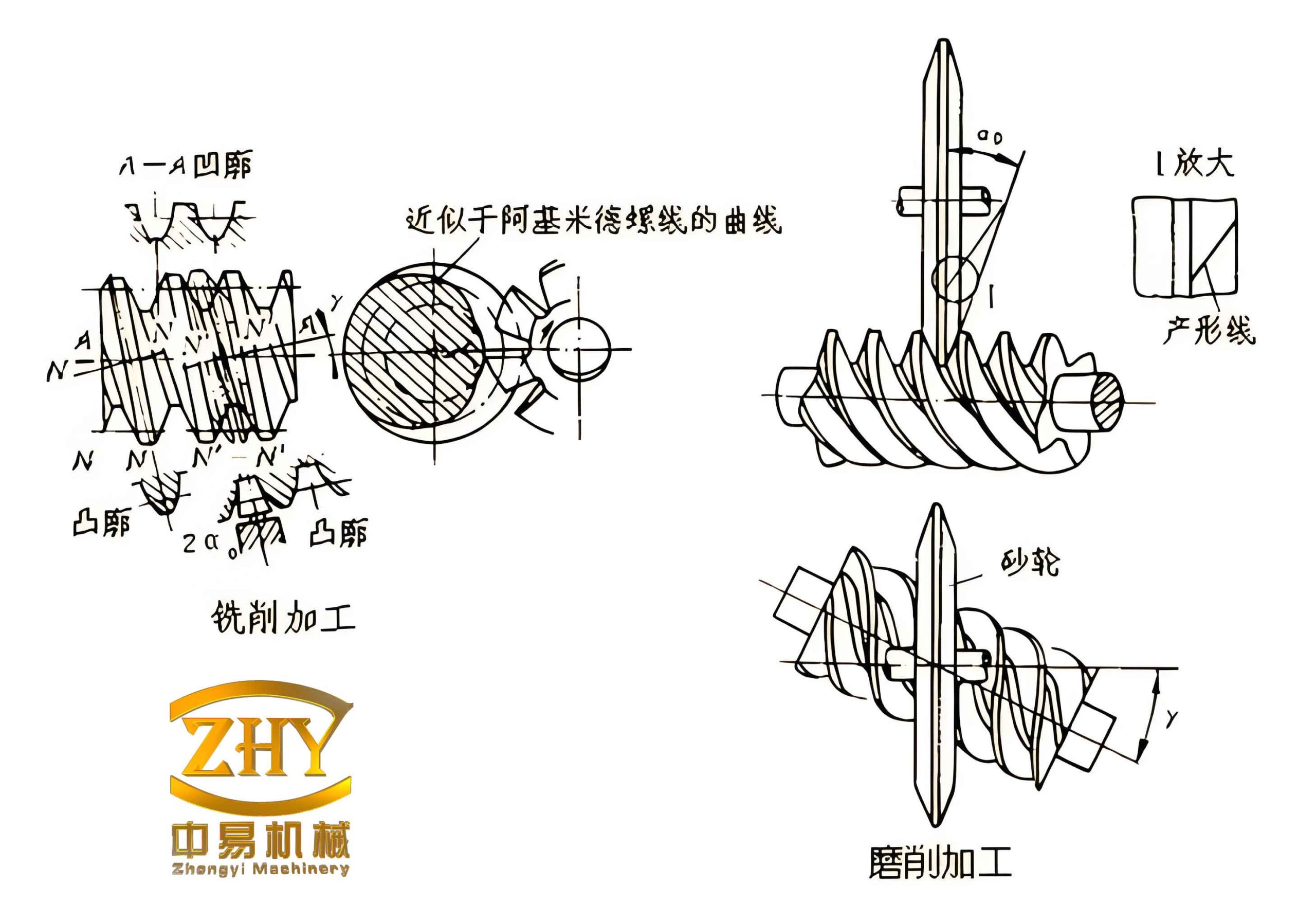
In an ideal dual-lead line-contact offset worm gear pair, the two tooth flanks of the worm are involute helicoids with different base circles and base helix angles. During manufacturing, straight-line cutting edges must lie in the tangent planes of the base cylinders, and each flank is machined separately. The worm wheel is cut using a specialized worm wheel hob on a gear hobbing machine. To simplify production, we approximate one of the involute helicoids of the worm with an Archimedean helicoid. The worm then becomes an Archimedes-type worm, which can be turned on a lathe using methods similar to conventional worm machining. Correspondingly, by the principle of conjugation, the worm wheel can be cut with a standard module gear hob. Thus, the resulting conical worm gear pair, constructed by engineering approximation, retains the characteristics and advantages of the dual-lead line-contact offset worm gear drive while being significantly easier to manufacture. We define this type of worm gear drive as a quasi dual-lead worm gear transmission. A quasi dual-lead worm gear pair is illustrated conceptually.
Engineering Approximation Method and Error Sources
When the worm wheel and worm are machined using the above approximation, the tooth flanks deviate from the ideal surfaces, resulting in tooth flank errors. Take the worm as an example: in an ideal dual-lead worm, both flanks are involute helicoids. Let Q and Q’ denote the tangent planes of the two base cylinders of the dual-lead worm, with base circle radii \(r_{b1}\) and \(r_{b2}\) respectively. The base helix angles are \(\beta_{b1}\) and \(\beta’_{b1}\). Consider two straight lines that intersect the z-axis and make angles \(\bar{\beta}_{b1}\) and \(\bar{\beta}’_{b1}\) with the oxy plane. When these lines undergo helical motions with leads \(P\) and \(P’\) around the z-axis, they generate two Archimedean helicoids \(\Sigma_1\) and \(\Sigma_2\) that form the two flanks of the quasi dual-lead worm.
The equation of \(\Sigma_1\) is:
$$ \begin{cases} x = t\cos\bar{\beta}_{b1}\cos\eta \\ y = t\cos\bar{\beta}_{b1}\sin\eta \\ z = t\sin\bar{\beta}_{b1} + \dfrac{P}{2\pi}\eta \end{cases} $$
Similarly, the equation of \(\Sigma_2\) is:
$$ \begin{cases} x = t_1\cos\bar{\beta}_{b1}\cos\eta_1 \\ y = t_1\cos\bar{\beta}_{b1}\sin\eta_1 \\ z = t_1\sin\bar{\beta}_{b1} + \dfrac{P}{2\pi}\eta_1 \end{cases} $$
where \(t, t_1, \eta, \eta_1\) are variable parameters. Setting \(y = r_{b2}\) in Eq. (1) (i.e., intersecting the Archimedean helicoid \(\Sigma_1\) with plane Q) yields the intersection curve \(\Gamma_1\). Its equation is:
$$ z = r_{b2}\tan\beta_{b1}\arctan\left(\frac{r_{b2}}{x}\right) + \frac{\tan\bar{\beta}_{b1}}{\sin\left[\arctan\left(\frac{r_{b2}}{x}\right)\right]} r_{b2}, \quad x \in (q\cdot r_{b2}, n\cdot r_{b2}) $$
If this curve \(\Gamma_1\) closely coincides with the straight line (the generating line of the involute helicoid) on plane Q within the meshing zone, then the Archimedean helicoid can be considered a valid approximation. The degree of coincidence is measured by the maximum perpendicular distance and the slope difference between the curve and the straight line.
Error Calculation
We calculate the external meshing error as an example. Referring to the geometric interpretation, we take two distinct points \((x_1, z_1)\) and \((x_2, z_2)\) on curve \(\Gamma_1\) and draw a chord \(L_1\). To simplify, we let \(Z = z\) and \(X = x\). The chord equation is:
$$ (Z – z_1)(X – x_1) = (z_1 – z_2)(x_1 – x_2) $$
Using iterative computation, we initially set \(x_1 = q\cdot r_{b2}\) and \(x_2 = n\cdot r_{b2}\). Substituting into Eq. (3) gives:
$$ (x_1, z_1) = \left(q r_{b2},\; \frac{r_{b2}}{\sin[\arctan(1/q)]}\tan\bar{\beta}_{b1} + r_{b2}\tan\beta_{b1}\arctan(1/q) \right) $$
$$ (x_2, z_2) = \left(n r_{b2},\; \frac{r_{b2}}{\sin[\arctan(1/n)]}\tan\bar{\beta}_{b1} + r_{b2}\tan\beta_{b1}\arctan(1/n) \right) $$
After several iterations, we obtain an optimal chord \(L_2\) that best approximates the curve \(\Gamma_1\). The slope of this chord is \(\tan\bar{\beta}_{b1}\) and is computed as:
$$ \tan\bar{\beta}_{b1} = \frac{z_1 – z_2}{x_1 – x_2} $$
Let the theoretical slope of the external meshing intersection line for the ideal dual-lead worm be \(\tan\beta_{b1}\). Then we define two error terms:
- External slope error \(\Delta_k\) – the absolute difference between the slope of chord \(L_2\) and the theoretical slope:
$$ \Delta_k = |\tan\bar{\beta}_{b1} – \tan\beta_{b1}| $$
- External distance error \(\Delta\) – half of the maximum absolute perpendicular distance from the chord \(L_2\) to the curve \(\Gamma_1\):
$$ \Delta = \frac{1}{2} \max_{X \in (q r_{b2}, n r_{b2})} \left| Z – z \right| \cos\bar{\beta}_{b1} $$
Similarly, internal meshing errors \(\Delta_k’\) and \(\Delta’\) can be computed. When both \(\Delta\) and \(\Delta’\) are sufficiently small (e.g., \(<10^{-2}\)) and \(\Delta_k\) and \(\Delta_k’\) are also below \(10^{-2}\), the two resulting involute helicoids with base radii \(r_{b2}\) and \(r’_{b2}\) and helix angles \(\bar{\beta}_{b1}\) and \(\bar{\beta}’_{b1}\) can be effectively replaced by the two Archimedean helicoids of the quasi dual-lead worm.
Worm Wheel Machining Error
Consider a right-handed quasi dual-lead worm wheel meshing with a left-handed quasi dual-lead worm. The worm wheel is cut using a left-handed cylindrical gear hob with module \(m\), outer diameter \(D\), axial tooth angle \(2a\), helix angle \(\gamma\), and number of starts = 1. The outer diameter \(D\) is set equal to the large-end diameter \(d_d\) of the quasi dual-lead worm, i.e., \(d_d = D\). To cut a worm wheel with \(z\) teeth and module \(m\) for a quasi dual-lead worm gear pair, the hob is installed with the same offset distance as in the transmission, and the cylindrical hob is rotated by an angle \(\theta\) equal to the cone angle of the quasi dual-lead worm. The geometric relationship gives \(\beta_{b1} = a – \theta\). Unlike conventional hobbing, the hob is positioned on the end face of the blank rather than the side. Because the worm wheel is cut using the principle of conjugation, and a standard cylindrical gear hob is used, there is no theoretical error in the worm wheel machining process—the tooth flank is generated exactly as required for the quasi dual-lead worm gear pair.
Manufacturing and Test Results
We manufactured two quasi dual-lead worm gear pairs with worm wheel tooth numbers of 70 and 410 (both with single-start worms). The calculated \(\Delta\) and \(\Delta’\) values, as well as \(\Delta_k\) and \(\Delta_k’\), were all below \(10^{-2}\). The worms and worm wheels were made of steel. To reduce the approximation errors, after cutting, the worm and worm wheel were subjected to conjugate lapping, which improved surface roughness and mesh quality. Test results confirmed that the quasi dual-lead worm gear transmission can be correctly manufactured and that it exhibits all the characteristics of conical worm gear drives and the advantages of dual-lead offset worm gear drives.
Based on our work, the following conclusions are drawn:
- The quasi dual-lead worm gear transmission replaces involute helicoids with Archimedean helicoids for the worm flanks, and using the principle of conjugation yields a compatible worm wheel tooth flank that retains the features of dual-lead offset worm gear drives.
- Tooth flank errors exist but are very small and can be further reduced by parameter adjustments and lapping. These errors do not significantly affect the transmission characteristics. The instantaneous meshing condition is approximately line contact.
- Experimental results demonstrate that the engineering approximation method is valid. The transmission runs smoothly, and manufacturing is simple: the worm wheel can be cut on a gear hobbing machine using a standard module gear hob, and the worm can be turned on a lathe using conventional Archimedes worm cutting techniques.
Summary of Key Formulas and Parameters
We summarize the main formulas used for error calculation in the following table.
| Symbol | Description | Formula |
|---|---|---|
| \(\Sigma_1\) | Archimedean helicoid for external flank | \(x = t\cos\bar{\beta}_{b1}\cos\eta,\; y = t\cos\bar{\beta}_{b1}\sin\eta,\; z = t\sin\bar{\beta}_{b1} + \frac{P}{2\pi}\eta\) |
| \(\Sigma_2\) | Archimedean helicoid for internal flank | \(x = t_1\cos\bar{\beta}_{b1}\cos\eta_1,\; y = t_1\cos\bar{\beta}_{b1}\sin\eta_1,\; z = t_1\sin\bar{\beta}_{b1} + \frac{P}{2\pi}\eta_1\) |
| \(\Gamma_1\) | Intersection curve of \(\Sigma_1\) with plane Q | \(z = r_{b2}\tan\beta_{b1}\arctan\left(\frac{r_{b2}}{x}\right) + \frac{\tan\bar{\beta}_{b1}}{\sin[\arctan(r_{b2}/x)]} r_{b2}\) |
| \(\tan\bar{\beta}_{b1}\) | Slope of optimal chord | \(\tan\bar{\beta}_{b1} = (z_1 – z_2)/(x_1 – x_2)\) |
| \(\Delta_k\) | External slope error | \(\Delta_k = |\tan\bar{\beta}_{b1} – \tan\beta_{b1}|\) |
| \(\Delta\) | External distance error | \(\Delta = \frac{1}{2} \max_{X} |Z – z| \cos\bar{\beta}_{b1}\) |
| \(\Delta_k’, \Delta’\) | Internal slope and distance errors (similar) | Analogous formulas with primed parameters |
Additionally, we provide a table summarizing the parameters of the two test worm gear pairs.
| Parameter | Pair 1 | Pair 2 |
|---|---|---|
| Worm wheel teeth \(z\) | 70 | 410 |
| Worm starts | 1 | 1 |
| Transmission ratio | 70 | 410 |
| Module \(m\) (mm) | Standard | Standard |
| External slope error \(\Delta_k\) | < \(10^{-2}\) | < \(10^{-2}\) |
| Internal slope error \(\Delta_k’\) | < \(10^{-2}\) | < \(10^{-2}\) |
| Distance error \(\Delta\) (mm) | < 0.01 | < 0.01 |
| Material | Steel | Steel |
The successful operation of these two pairs confirms that the quasi dual-lead worm gear transmission is a practical and efficient solution for applications requiring large ratio, smooth motion, and ease of manufacturing. The engineering approximation method introduced here bridges the gap between theoretical precision and manufacturing feasibility, making advanced worm gear drives accessible for a wider range of industrial uses.