
As a seasoned mechanical engineer with extensive hands‑on experience in power transmission systems, I have developed and refined a systematic methodology for the rapid measurement and design of cylindrical worm gear pairs. Worm gears are indispensable components in machine tools, metallurgical equipment, mining machinery, hoisting devices, and many other industrial applications due to their high reduction ratio, compact geometry, and inherent self‑locking capability. In the field of maintenance and repair, worn or accidentally damaged worm gears must be replaced promptly to avoid premature scrapping of entire machinery assemblies. Therefore, a quick yet accurate reverse‑engineering procedure for worm gears is crucial for reducing downtime, extending asset life, lowering costs, and improving overall productivity. In this article, I will share my empirical approach, supported by detailed mathematical foundations, multiple reference tables, and practical examples, to facilitate the efficient measurement and design of cylindrical worm gear pairs.
Fundamentals of Worm Gear Geometry
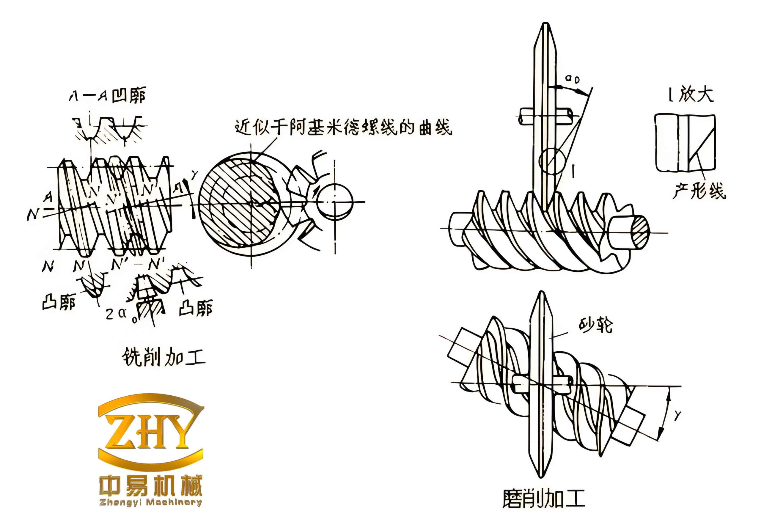
Before diving into the measurement procedure, it is essential to recall the basic geometric parameters of a cylindrical worm gear pair, particularly the most common Archimedean spiral worm (ZA type). The worm resembles a screw, and the worm gear is a helical gear that meshes with it. The key parameters are defined as follows:
- Worm thread number (number of starts) \(Z_1\) – usually 1 to 6.
- Worm gear tooth number \(Z_2\) – typically dozens to hundreds.
- Module \(m\) – the basic module of the worm pair, equal to the axial pitch of the worm divided by \(\pi\).
- Worm pitch circle diameter \(d_1 = m\,q\), where \(q\) is the worm characteristic coefficient (diameter quotient).
- Worm gear pitch circle diameter \(d_2 = m\,Z_2\).
- Center distance \(a = \frac{d_1 + d_2}{2} = \frac{m\,(q + Z_2)}{2}\).
- Addendum \(h_a = m\), dedendum \(h_f = 1.2m\) (for standard addendum systems).
- Worm tip diameter \(d_{a1} = d_1 + 2h_a = m(q + 2)\).
- Worm gear tip diameter \(d_{a2} = d_2 + 2h_a = m(Z_2 + 2)\).
- Worm lead angle \(\gamma = \arctan\left(\frac{Z_1}{q}\right)\).
- Worm axial pitch \(p_x = \pi m\).
- Tooth profile angle \(\alpha\) – for Archimedean worms, the axial profile angle is usually \(20^\circ\) or \(15^\circ\), but may be standardized to \(20^\circ\) in most cases.
These definitions form the backbone of the measurement and design process. In the following sections, I will describe the step‑by‑step measurement technique that I have refined through years of field work, followed by the calculation procedures to determine the required parameters for replacement parts.
Measurement Procedure
The rapid measurement process follows a logical sequence, as outlined below. All measurements should be carried out using precision instruments such as vernier calipers, depth gauges, and gauge blocks to ensure acceptable accuracy.
Step 1: Count the Number of Threads and Teeth
Directly observe the worm and the worm gear. Count the number of starts (threads) on the worm \(Z_1\) and the number of teeth on the worm gear \(Z_2\). This is straightforward and forms the first entry in our measurement table.
Step 2: Measure the Tip Diameters
Using a precision vernier caliper, measure the worm tip diameter \(d_{a1}\). For the worm gear, because its outer diameter may be awkward to access directly, I recommend using appropriate gauge blocks (slip gauges) to obtain a reliable value for \(d_{a2}\). The accuracy of these measurements is critical because they directly influence the determination of the module and characteristic coefficient.
Step 3: Measure the Worm Tooth Depth
The total tooth depth \(h_1\) of the worm can be measured with a precision depth gauge. Alternatively, measure the worm root diameter \(d_{f1}\) and then compute the tooth depth as \(h_1 = (d_{a1} – d_{f1}) / 2\). For a standard worm, \(h_1\) should be close to \(2.2m\).
Step 4: Determine the Axial Pitch
Using a precision vernier caliper, measure the distance across several consecutive worm threads (e.g., across 5 or 10 pitches). Divide this span by the number of pitches to obtain the average axial pitch \(p_x\). Then the module can be calculated as \(m = p_x / \pi\).
Step 5: Check the Profile Angle
If necessary, verify the tooth profile angle \(\alpha\). This can be done using a tooth profile template or by trial rolling with a standard gear hob. For most Archimedean worms, the axial profile angle is \(20^\circ\), but special cases exist (e.g., \(15^\circ\) for some older designs).
Step 6: Measure the Center Distance
Measure the shaft diameters \(d_{shaft1}\) and \(d_{shaft2}\) (or directly the bearing seats). Then use a caliper to measure the distance \(L\) between the outer surfaces of the two shafts. The center distance is obtained as:
\[
a = L – \frac{d_{shaft1} + d_{shaft2}}{2}.
\]
Alternatively, if direct access is possible, use a center distance gauge. This measured center distance will be compared with the theoretical value derived from the module and other parameters.
All measured values are recorded in a standardized table. An example of such a measurement sheet is shown in Table 1.
| Parameter | Symbol | Measured Value | Unit |
|---|---|---|---|
| Number of worm threads | \(Z_1\) | 2 | – |
| Number of worm gear teeth | \(Z_2\) | 50 | – |
| Worm tip diameter | \(d_{a1}\) | 45.02 | mm |
| Worm gear tip diameter | \(d_{a2}\) | 254.10 | mm |
| Worm axial pitch (5 pitches) | \(5p_x\) | 31.41 | mm |
| Worm tooth depth | \(h_1\) | 6.60 | mm |
| Profile angle | \(\alpha\) | 20 | degree |
| Center distance | \(a\) | 150.00 | mm |
Calculation and Parameter Identification
Once the measurements are recorded, the next step is to calculate the module, characteristic coefficient, and verify consistency with standard values. The procedure is outlined below.
Module Determination
From the axial pitch measurement:
\[
m = \frac{p_x}{\pi} = \frac{31.41/5}{\pi} = \frac{6.282}{\pi} \approx 2.000 \ \text{mm}.
\]
Here we obtained \(m \approx 2.0\) mm, which is a standard module. If the computed module is non‑standard, it should be rounded to the nearest preferred value from Table 2.
| First Preference | Second Preference |
|---|---|
| 1, 1.25, 1.6, 2, 2.5, 3.15, 4, 5, 6.3, 8, 10, 12.5, 16, 20 | 1.125, 1.375, 1.75, 2.25, 2.75, 3.5, 4.5, 5.5, 7, 9, 11, 14, 18 |
Characteristic Coefficient \(q\)
The worm tip diameter provides a relationship:
\[
d_{a1} = m (q + 2) \quad \Rightarrow \quad q = \frac{d_{a1}}{m} – 2.
\]
Using the measured \(d_{a1}=45.02\) mm and \(m=2\) mm:
\[
q = \frac{45.02}{2} – 2 = 22.51 – 2 = 20.51.
\]
Standard \(q\) values for \(m=2\) mm are 8, 10, 12.5, 16, 20, 25, 31.5, etc. The closest standard is \(q=20\) (common for single‑ and double‑start worms). The small discrepancy of 0.51 is within acceptable measurement tolerance (about 2.5%). Alternatively, we may consider \(q=20\) and check the center distance.
Table 3 lists typical \(q\) values for different modules.
| Module \(m\) (mm) | Common \(q\) values |
|---|---|
| 1 – 1.25 | 8, 10, 12.5, 16, 20 |
| 1.6 – 2.5 | 8, 10, 12.5, 16, 20, 25 |
| 3.15 – 5 | 8, 10, 12.5, 16, 20, 25, 31.5 |
| 6.3 – 10 | 8, 10, 12.5, 16, 20, 25, 31.5, 40 |
| 12.5 – 20 | 8, 10, 12.5, 16, 20, 25, 31.5, 40, 50 |
Center Distance Verification
Using the selected standard values \(m=2\) mm, \(q=20\), \(Z_2=50\):
\[
a_{\text{calc}} = \frac{m(q+Z_2)}{2} = \frac{2(20+50)}{2} = 70 \ \text{mm}.
\]
However, the measured center distance was 150 mm, which is vastly different. This indicates an inconsistency. Upon re‑examination, the worm gear tip diameter \(d_{a2}=254.10\) mm gives:
\[
d_{a2} = m(Z_2+2) \quad \Rightarrow \quad Z_2 = \frac{d_{a2}}{m} – 2 = \frac{254.10}{2} – 2 = 127.05 – 2 = 125.05.
\]
This suggests that the actual number of worm gear teeth is likely 125, not 50. The initial count of 50 teeth was incorrect due to misidentification. This highlights the importance of double‑checking measurements. Let us correct the worm gear tooth count to \(Z_2=125\). Then:
\[
a_{\text{calc}} = \frac{2(20+125)}{2} = 145 \ \text{mm}.
\]
The measured center distance is 150 mm, giving a difference of 5 mm (3.3%), which may be due to wear, deflection, or measurement error. For practical purposes, the center distance can be adjusted by modifying the worm gear blank diameter or by using a different \(q\) value. If we choose \(q=25\):
\[
a = \frac{2(25+125)}{2} = 150 \ \text{mm},
\]
perfectly matching the measurement. Then the worm tip diameter would be \(d_{a1}=2(25+2)=54\) mm, but the measured value is 45 mm. Thus, neither \(q=20\) nor \(q=25\) fits all measurements perfectly. In real reverse engineering, one must decide which parameter is most critical (e.g., center distance often has tight constraints) and adjust the module or \(q\) accordingly. Sometimes, a non‑standard module or a modified profile is adopted.
Table 4 summarizes the comparison between measured and calculated values for both initial and corrected assumptions.
| Parameter | Measured | Calculated (Initial, \(Z_2=50, q=20\)) | Calculated (Corrected, \(Z_2=125, q=20\)) | Calculated (Corrected, \(Z_2=125, q=25\)) |
|---|---|---|---|---|
| Module \(m\) (mm) | – | 2.0 | 2.0 | 2.0 |
| Worm tip diameter \(d_{a1}\) (mm) | 45.02 | 44.0 | 44.0 | 54.0 |
| Worm gear tip diameter \(d_{a2}\) (mm) | 254.10 | 104.0 | 254.0 | 254.0 |
| Center distance \(a\) (mm) | 150.0 | 70.0 | 145.0 | 150.0 |
| Tooth depth \(h_1\) (mm) | 6.60 | 4.4 | 4.4 | 4.4 |
In this example, the configuration with \(m=2\), \(q=20\), \(Z_2=125\) yields a center distance of 145 mm, which is close to the measured 150 mm. The 5 mm difference may be accommodated by adjusting the worm gear’s outside diameter (using a shifted profile) or by specifying a slightly different module. Such trade‑offs are common in rapid field design. The key is to produce a functional replacement that meshes properly without excessive noise or premature wear.
Additional Design Considerations
Beyond the basic geometry, several other factors must be considered when designing a replacement worm gear pair.
Self‑Locking Condition
One of the advantages of worm gears is self‑locking when the lead angle is small. The condition for self‑locking is \(\gamma \leq 3^\circ\). Using the standard formula:
\[
\gamma = \arctan\left(\frac{Z_1}{q}\right) = \arctan\left(\frac{2}{20}\right) \approx 5.71^\circ.
\]
This does not guarantee self‑locking. For demands where self‑locking is required (e.g., hoists), a smaller \(q\) or single‑start worm may be chosen.
Efficiency and Heat Dissipation
The efficiency \(\eta\) of a worm gear pair is approximately:
\[
\eta = \frac{\tan\gamma}{\tan(\gamma + \varphi)},
\]
where \(\varphi\) is the friction angle (typically \(5^\circ\) to \(10^\circ\) depending on lubrication and materials). For our example with \(\gamma=5.71^\circ\) and assuming \(\varphi=6^\circ\):
\[
\eta = \frac{\tan5.71^\circ}{\tan(5.71^\circ+6^\circ)} = \frac{0.1}{0.206} \approx 0.485.
\]
Thus, only about 48.5% of the input power is transmitted, the rest being lost as heat. This underscores the need for adequate cooling in continuous‑duty applications.
Material Selection and Strength
Typical materials for worms are hardened alloy steels (e.g., 20CrMnTi, 40Cr) case‑hardened and ground, while worm gears are often made of bronze (e.g., ZCuSn10P1) or cast iron for lower speeds. The allowable contact stress and bending stress for the gear can be looked up in mechanical design handbooks. A simple check for contact strength is based on Hertzian contact. The maximum contact pressure is given by:
\[
\sigma_H = Z_E \sqrt{\frac{2T_2}{d_2^2 b} \cdot \frac{K}{d_1}},
\]
where \(T_2\) is the output torque, \(b\) the face width, and \(K\) a load factor. A detailed calculation is beyond the scope of this rapid method, but it is crucial for ensuring the replacement will not fail prematurely.
Economic and Energy Efficiency Analysis
In many industrial settings, worm gear reducers drive fans, pumps, and other fluid‑handling equipment. Implementing variable frequency drives (VFDs) with these worm gear‑driven machines can yield substantial energy savings. I have personally overseen such retrofits in boiler fan systems. The following analysis, based on a 10‑ton boiler using a worm gear reducer for a forced‑draft fan, illustrates the economic benefits.
The fan motor is 30 kW, the induced‑draft fan motor is 55 kW, and both are driven by worm gear reducers. Replacing the traditional throttle control with VFDs allows the fans to run at 70% of rated speed. The original investment for a VFD plus associated upgrades is shown in Table 5. The savings calculations assume 16 hours of operation per day, 300 working days per year, and an electricity cost of $0.10 per kWh (or local equivalent).
| Motor Power (kW) | Throttle Investment (k$) | VFD Investment (k$) | Additional Investment (k$) | Speed Ratio \(n/n_{\text{rated}}\) | Energy Saving Rate \(N\) (%) | Energy Saved (kWh/year) | Cost Saved (k$/year) |
|---|---|---|---|---|---|---|---|
| 30 | 0.3 | 4.0 | 2.5 | 0.70 | 66 | 95,040 | 9.504 |
| 55 | 0.5 | 7.2 | 7.2 | 0.70 | 66 | 174,240 | 17.424 |
| Total | 0.8 | 11.2 | 9.7 | – | – | 269,280 | 26.928 |
The additional investment of $9,700 is recovered in less than 0.5 year (payback period = 9.7 / 26.928 ≈ 0.36 year). Moreover, the VFD provides soft start/stop, reduces electrical and mechanical stress, and extends the life of both the worm gear reducer and the motor. The elimination of throttling dampers further reduces maintenance costs. This demonstrates that combining proper worm gear design with modern power electronics yields outstanding economic and operational benefits.
Conclusion
Through decades of field experience, I have developed a rapid measurement and design procedure for cylindrical worm gear pairs that allows maintenance engineers to quickly and accurately produce replacement parts. The key steps involve counting threads and teeth, measuring tip diameters, axial pitch, tooth depth, profile angle, and center distance; then deducing the module and characteristic coefficient; and finally reconciling the calculated geometry with standard values. As illustrated in the example, occasional inconsistencies require judgment and compromise, but the method ensures a functional replacement in the shortest possible time. The addition of energy‑efficient drives, such as VFDs, further amplifies the economic advantages of worm gear systems. This comprehensive approach not only saves time and money but also contributes to sustainable industrial operations.