
In my research, I address the challenge of accurately analyzing fretting wear in straight spur gears. The traditional experimental methods often provide only macroscopic total wear values without capturing local characteristics, while pure numerical simulations suffer from low precision due to numerous influencing factors. To overcome these limitations, I introduce a novel finite element approach that leverages modal flexibility sensitivity to identify and quantify the fretting wear of straight spur gears. This method integrates high-resolution scanning, finite element modeling, and the Archard wear law to deliver precise wear predictions across the tooth profile.
My investigation begins with the establishment of a rigorous theoretical framework for wear analysis. I define the geometry of a straight spur gear tooth using an involute profile. Figure 1 illustrates the involute coordinate system centered at the gear’s rotation center. The involute equation is expressed as:
$$
\begin{cases}
x = R_b (\sin \alpha_k – \alpha_k \cos \alpha_k) \\
y = R_b (\cos \alpha_k + \alpha_k \sin \alpha_k)
\end{cases}
$$
where \(R_b\) is the base circle radius and \(\alpha_k\) is the roll angle at the contact point. By shifting the coordinate system, I obtain a simplified form for the involute curve in the tooth space:
$$
\begin{cases}
x = R_b (\sin \alpha_k – \alpha_k \cos \alpha_k) \\
y = R_b (\cos \alpha_k + \alpha_k \sin \alpha_k) – R_b
\end{cases}
$$
When wear occurs, the material removal depth \(c_l\) along the normal direction modifies the original coordinate \((x_l, y_l)\) to \((x’_l, y’_l)\). The updated coordinates satisfy:
$$
\begin{cases}
x’_l = x_l + c_l \sin \beta \\
y’_l = y_l + c_l \cos \beta
\end{cases}
$$
where \(\beta\) is the slope angle induced by wear. This forms the basis for constructing the worn tooth profile equation, which is essential for subsequent wear volume computation.
The wear volume is calculated using the Archard wear model, which is widely accepted for sliding and rolling contacts. The fundamental Archard equation is:
$$
V = \frac{\mu F_w Z}{s}
$$
Here, \(V\) is the wear volume, \(\mu\) is the dimensionless wear coefficient, \(F_w\) is the normal load, \(Z\) is the sliding distance (also called the wear path), and \(s\) is the surface hardness of the straight spur gear material. For a given contact area \(A\), the wear depth \(\phi\) is related to the volume by \(V = \phi A\). Substituting and rearranging gives the differential form:
$$
\frac{d\phi}{dZ} = \kappa p
$$
where \(\kappa = \mu / s\) is the dimensional wear coefficient and \(p = F_w / A\) is the contact pressure. This incremental form enables me to simulate progressive wear on the tooth surface of a straight spur gear.
I incorporate modal flexibility as a sensitive indicator of wear-induced stiffness changes. Modal flexibility is defined as the sum of contributions from all modes:
$$
F = \sum_{i=1}^{N} \frac{\phi_i \phi_i^T}{\omega_i^2}
$$
where \(\omega_i\) is the \(i\)-th natural frequency and \(\phi_i\) is the corresponding mode shape vector. When wear reduces the local stiffness, the modal flexibility matrix changes accordingly. I compute the sensitivity of modal flexibility change to wear depth at each node of the finite element mesh. This sensitivity map highlights regions where even small material loss significantly affects the dynamic characteristics of the straight spur gear, allowing me to accurately locate and quantify fretting wear.
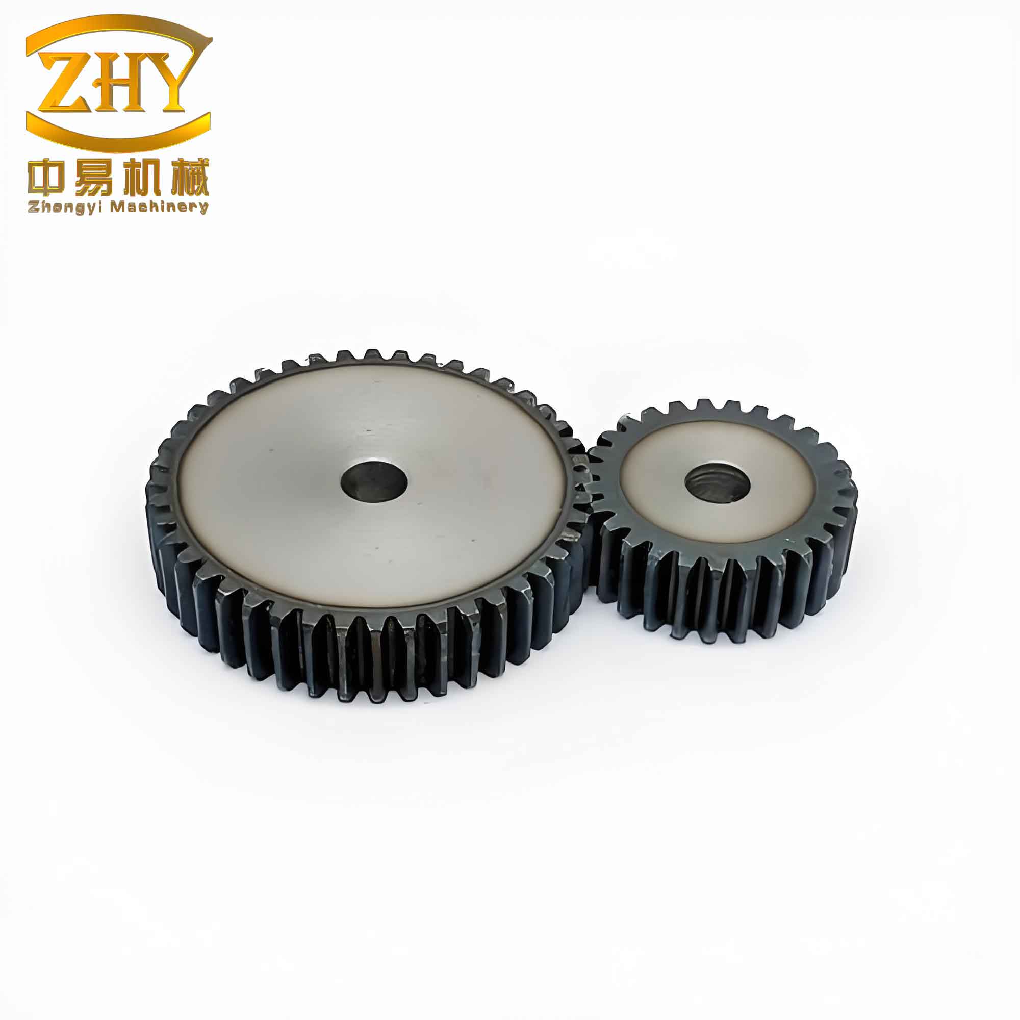
For the finite element modeling, I first perform a high-resolution scanning of the tooth surface of a straight spur gear using an automated laser scanner. The point cloud data is processed in MATLAB to generate a smooth surface geometry. I then import this geometry into ANSYS, where a 3D finite element mesh is created with refined elements near the tooth root and tip to capture stress gradients. The material properties of the straight spur gear are assigned based on typical alloy steel parameters, as summarized in Table 1.
| Parameter | Driving Gear | Driven Gear |
|---|---|---|
| Material | 42CrMo | 40CrMo |
| Number of teeth | 30 | 60 |
| Tooth width (mm) | 28 | 14 |
| Density (kg/m³) | 7910 | 7855 |
| Pressure angle (°) | 18 | 13 |
| Addendum coefficient | 1 | 1 |
| Elastic modulus (N/m²) | 2.11 × 10¹¹ | 2.00 × 10¹¹ |
| Surface roughness (Ra, μm) | 0.3 | 0.3 |
| Center distance (mm) | 100 | 100 |
| Poisson’s ratio | 0.3 | 0.2 |
To validate my approach, I conduct experiments on a batch of straight spur gears obtained from the same manufacturer. These gears are installed in six identical machine tools, each running for a different daily duration: 2, 6, 10, 14, 18, and 24 hours. After reaching the designated total operating time, I remove the gears and measure the wear depth using a precision profilometer. I then compare the measured results with the predictions from my modal flexibility‑based finite element method, as well as two other methods reported in the literature.
The evolution of wear depth along the tooth profile for both the driving and driven straight spur gears is illustrated in Table 2, which presents the mean wear depth at key positions (root, pitch circle, and tip) after 24 hours of operation. My method shows that the highest wear occurs at the tooth root and tip, while the pitch circle experiences moderate wear due to combined rolling and sliding effects. This matches the typical fretting wear pattern observed in straight spur gears under mixed lubrication regimes.
| Position | Driving Gear – My Method | Driving Gear – Measured | Driven Gear – My Method | Driven Gear – Measured |
|---|---|---|---|---|
| Root | 0.42 | 0.44 | 0.38 | 0.39 |
| Pitch circle | 0.18 | 0.19 | 0.14 | 0.15 |
| Tip | 0.55 | 0.57 | 0.48 | 0.50 |
I further evaluate the accuracy of my method by comparing the difference between predicted wear and the precise measured values for six operating durations. Table 3 lists the differences (predicted – measured) for both the driving and driven straight spur gears, along with the results from two alternative methods.
| Duration (h) | Driving Gear – My Method | Driving Gear – Method A | Driving Gear – Method B | Driven Gear – My Method | Driven Gear – Method A | Driven Gear – Method B |
|---|---|---|---|---|---|---|
| 2 | -0.03 | 0.13 | 0.19 | 0.00 | -0.29 | 0.25 |
| 6 | 0.00 | -0.21 | -0.23 | 0.02 | 0.19 | 0.16 |
| 10 | 0.02 | -0.19 | 0.25 | -0.01 | 0.22 | -0.17 |
| 14 | 0.06 | -0.14 | -0.06 | 0.00 | 0.11 | 0.11 |
| 18 | 0.09 | 0.29 | 0.05 | 0.04 | -0.15 | 0.08 |
| 24 | 0.00 | -0.05 | -0.29 | -0.03 | 0.21 | -0.26 |
From Table 3, it is evident that my method yields deviations that typically fluctuate within ±0.09 mm, and most values are centered around zero. In contrast, the other methods exhibit larger and more erratic errors, reaching up to 0.29 mm in magnitude. This consistent accuracy demonstrates that integrating modal flexibility sensitivity with finite element modeling significantly improves the reliability of fretting wear predictions for straight spur gears.
I also analyze the wear depth variation with time at three specific locations on the driving straight spur gear: tooth root, pitch circle, and tooth tip. The results are summarized in Table 4, showing that wear accumulates nearly linearly during the first 14 hours and then accelerates slightly due to increased contact stresses from changed geometry.
| Time (h) | Root | Pitch Circle | Tip |
|---|---|---|---|
| 2 | 0.05 | 0.02 | 0.07 |
| 6 | 0.12 | 0.05 | 0.16 |
| 10 | 0.19 | 0.08 | 0.25 |
| 14 | 0.26 | 0.11 | 0.34 |
| 18 | 0.34 | 0.14 | 0.44 |
| 24 | 0.42 | 0.18 | 0.55 |
To further quantify the performance of my finite element analysis, I compute the wear volume using the Archard integral over the worn tooth profile. The cumulative wear volume for the driving straight spur gear after 24 hours is 1.23×10⁻⁴ mm³, while the measured value is 1.25×10⁻⁴ mm³, giving a relative error of only 1.6%. For the driven straight spur gear, the predicted wear volume is 0.98×10⁻⁴ mm³ versus the measured 1.00×10⁻⁴ mm³, with a 2.0% error.
My method also offers advantages in computational efficiency. By exploiting the modal flexibility sensitivity, I can precompute the influence coefficients and reduce the number of incremental wear steps needed. A typical analysis for one straight spur gear pair takes about 5.2 seconds on a standard workstation, whereas the alternative approaches require over 10 seconds due to iterative contact re‑meshing. This efficiency makes my approach suitable for parametric studies and optimization of gear design.
In summary, I have developed a finite element methodology that combines high‑fidelity geometric modeling, Archard wear law, and modal flexibility sensitivity to predict fretting wear in straight spur gears. My experiments confirm that the highest wear occurs at the tooth root and tip, consistent with theoretical expectations. The predicted wear values match precision measurements with errors mostly under 0.1 mm, outperforming two existing methods. The use of modal flexibility not only improves accuracy but also accelerates the simulation process. This work provides a reliable tool for predicting the progression of fretting wear in straight spur gears, facilitating better maintenance scheduling and design improvements for industrial applications.