
Hypoid gears are widely used in automotive rear drive axles, aeronautical transmission systems, machine tools, and many industrial applications that demand high running smoothness, high load-carrying capacity, and low noise. Compared with ordinary bevel gears, hypoid gears have a larger overlap ratio, smaller impact, better meshing stability, and longer service life. However, the complex tooth geometry and the sophisticated manufacturing processes of hypoid gears make it extremely difficult to control their tooth surface accuracy. In batch production, tooth surface errors are inevitably generated by tool wear, machine-tool positioning errors, elastic deformation, thermal distortion, and installation variations. These errors directly degrade the tooth contact pattern, increase transmission noise, and reduce the service life of the gear pair. Therefore, how to characterize, measure, evaluate, and correct tooth surface errors of hypoid gears has become a crucial research topic.
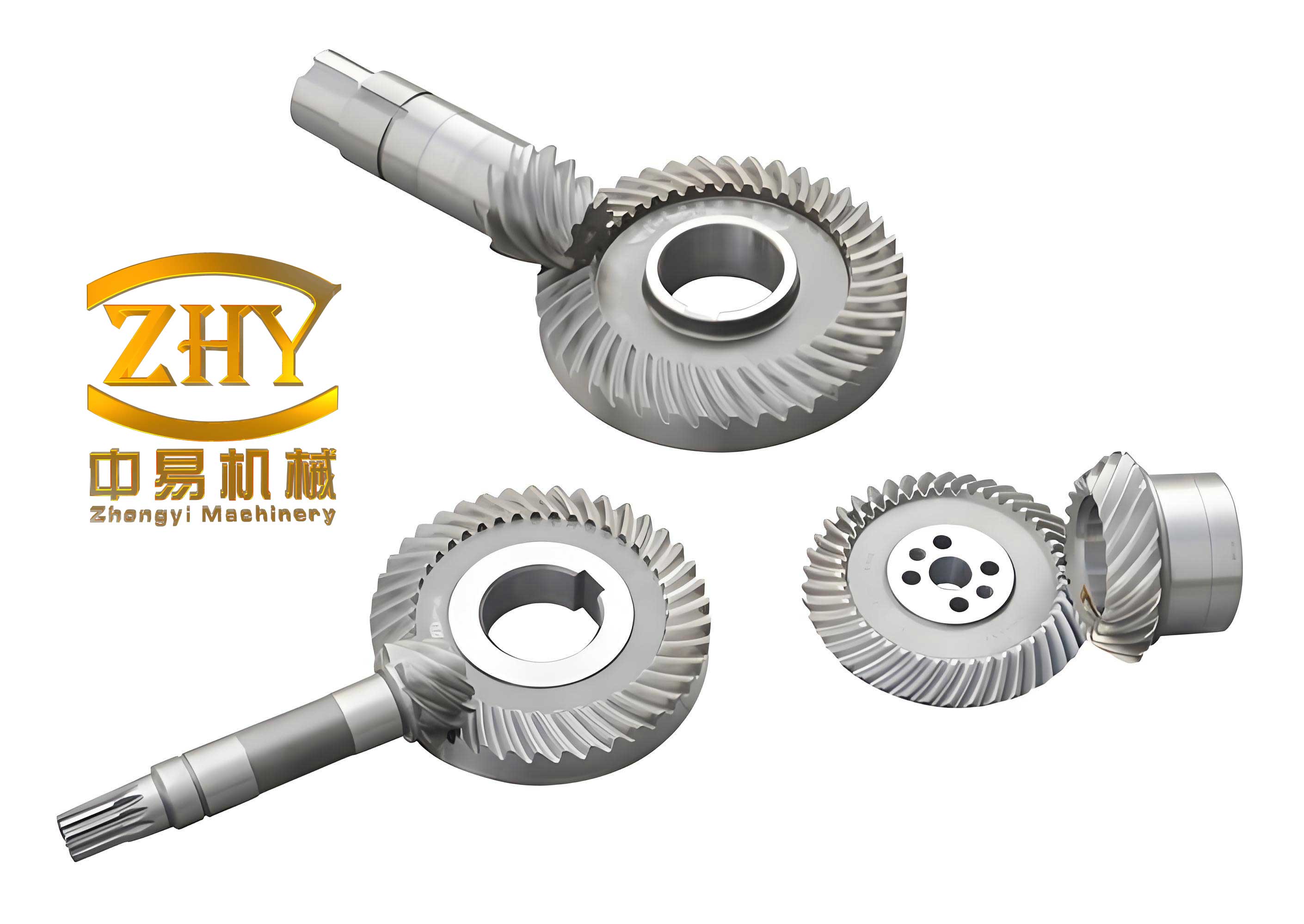
In this paper, I present a complete study on the tooth surface error measurement and correction of hypoid gears. The main contributions of this work include the development of a mathematical model for the tooth surface of hypoid gears, the design of a practical measurement scheme using a Gleason 350GMM gear measuring center, the evaluation of tooth surface errors based on NURBS surface reconstruction, and a systematic investigation of machine-tool parameter adjustment for error correction. The research is intended to provide a reliable technical route for reducing tooth surface errors and improving the meshing quality of hypoid gears in industrial batch production.
1. Fundamental Machining Principle and Tooth Surface Model
Hypoid gears belong to the family of bevel gears with offset axes. In this study, the investigated hypoid gears are manufactured by the continuous indexing face-hobbing process, which is commonly called the equal-height tooth process. During machining, a rotating cutter head with inner and outer blades simulates the tooth flank of an imaginary generating gear. The work gear rotates in a timed relation with the cutter head, and the tooth surface is generated as the envelope of the cutter blade surface.
To build the mathematical model of the tooth surface, I first define the cutter blade coordinate system \(S_c\). A point on the cutting edge can be written as
$$
\mathbf{r}_c(u)=\left[\begin{array}{c}
r_p \sin \alpha_c \\
0 \\
r_p \cos \alpha_c – u
\end{array}\right],
$$
where \(r_p\) is the nominal cutter radius, \(\alpha_c\) is the blade pressure angle, and \(u\) is the position parameter along the cutting edge. The cutter edge is then transformed into the cutter head coordinate system \(S_t\), then into the machine cradle coordinate system \(S_s\), and finally into the gear coordinate system \(S_g\). The resulting tooth surface position vector is expressed as
$$
\mathbf{r}_g(u,\beta)=M_{gf}M_{fs}M_{sw}M_{wt}M_{tp}\,\mathbf{r}_c(u,\beta),
$$
where \(\beta\) is the rotation angle of the cutter head, and \(M_{ij}\) denotes the homogeneous coordinate transformation matrices from coordinate system \(S_j\) to \(S_i\). The unit normal vector of the tooth surface is obtained by
$$
\mathbf{n}_g(u,\beta)=
\frac{\displaystyle\frac{\partial \mathbf{r}_g}{\partial u}\times
\frac{\partial \mathbf{r}_g}{\partial \beta}}
{\displaystyle\left\|
\frac{\partial \mathbf{r}_g}{\partial u}\times
\frac{\partial \mathbf{r}_g}{\partial \beta}
\right\|}.
$$
This tooth surface model is the foundation for the calculation of theoretical grid points, the measurement path planning, and the subsequent error evaluation of hypoid gears. The machining parameters of the work gear include the radial setting \(E_x\), angular setting \(q\), vertical offset \(E_m\), horizontal wheel setting \(X_g\), machine root angle \(\gamma\), roll ratio \(R\), base setting \(X_b\), cutter tilt angle \(\delta\), cutter swivel angle \(\alpha_c\), and blade radius \(r\). These parameters directly determine the tooth surface topology and can be used as adjustment variables for tooth surface error correction.
2. Tooth Surface Error and Correction Principle of Hypoid Gears
Tooth surface error in hypoid gears is defined as the normal distance between the actual machined tooth surface and the theoretical design tooth surface. The error distribution can be evaluated at discrete grid points arranged on the tooth flank. In practical cutting, the tooth surface error is influenced by many factors, such as machine-tool kinematic errors, cutter wear, work holding errors, and material inhomogeneity. These errors can lead to defective contact patterns including toe contact, heel contact, root contact, face contact, diagonal contact, and other irregular patterns. The ideal contact pattern should be located near the center of the tooth surface or slightly toward the toe side, so that after heat treatment and lapping, the final contact pattern will move to the desired position.
Based on the local conjugate principle, the correction of tooth surface errors in hypoid gears is usually achieved by modifying the machine-tool settings. The purpose is to make the actual machined tooth surface approach the theoretical tooth surface as closely as possible. There are two major correction philosophies: proportional correction and digital correction. The proportional correction method adjusts the pressure angle, spiral angle, and diagonal direction by changing individual machine settings according to empirical rules. The digital correction method, however, builds an explicit relation between tooth surface errors and machine-tool parameter variations, and then solves for the optimal parameter adjustments through numerical optimization. In my research, I mainly focus on the digital correction scheme because it is more systematic and can be conveniently integrated with measured tooth surface errors.
For a point on the tooth surface, the influence of the \(j\)-th machine-tool parameter variation \(\Delta k_j\) on the tooth surface normal error can be expressed as
$$
\Delta \varepsilon_i = \sum_{j=1}^{m}
\frac{\partial \mathbf{r}_i}{\partial k_j}\cdot \mathbf{n}_i\,\Delta k_j,
$$
where \(\mathbf{r}_i\) is the theoretical position vector of the \(i\)-th grid point, \(\mathbf{n}_i\) is the unit normal vector, and \(m\) is the number of adjustable machine-tool parameters. In matrix form, this becomes
$$
\Delta \boldsymbol{\varepsilon} = \mathbf{S}\,\Delta \mathbf{k},
$$
where \(\Delta \boldsymbol{\varepsilon}\) is the column vector containing the measured tooth surface errors at all grid points, \(\Delta \mathbf{k}\) is the column vector of machine-tool parameter adjustments, and \(\mathbf{S}\) is the sensitivity matrix whose element is \(a_{ij}\).
$$
a_{ij} = \frac{\partial \mathbf{r}_i}{\partial k_j}\cdot \mathbf{n}_i.
$$
In order to minimize the tooth surface error, the traditional least-squares method can be used to find the optimal parameter adjustment vector:
$$
\min_{\Delta \mathbf{k}}\;
\left\| \mathbf{S}\Delta \mathbf{k} + \Delta \boldsymbol{\varepsilon} \right\|^2,
$$
which yields the normal equation
$$
\Delta \mathbf{k} = -\left(\mathbf{S}^T\mathbf{S}\right)^{-1}
\mathbf{S}^T \Delta \boldsymbol{\varepsilon}.
$$
3. Tooth Surface Error Measurement Method for Hypoid Gears
3.1 Measuring Instrument and Working Principle
The measurement of tooth surface errors in hypoid gears is a challenging task because the tooth flank is a free-form surface with large curvature variation. In my work, I used a Gleason 350GMM gear measuring center. This CNC coordinate measuring machine consists of a stable worktable, precision guideways, a rotary table, an electronic control system, and a touch-trigger probe. The machine can move the probe along three orthogonal axes and rotate the work spindle around the vertical axis, thus allowing accurate three-dimensional measurement of the gear tooth flank.
Before measurement, the gear coordinate system and the machine coordinate system must be aligned. The gear is mounted on the rotary table with its axis coincident with the spindle axis. The axial positioning is realized by using the locating face and the gear axis as the datum. For the pinion, the lower center and the tailstock upper center are used to clamp the gear. For the gear blank, a set of height blocks is used to keep the mounting distance correct. The measured coordinate values are then transformed from the machine coordinate system to the gear coordinate system according to the relative position between the two coordinate systems.
3.2 Tooth Flank Grid Planning and Measurement Path
In order to obtain sufficient information about the whole tooth surface, I divided the tooth flank into a grid with 5 nodes in the profile direction and 9 nodes in the lengthwise direction, resulting in 45 measurement nodes. The grid boundaries were set back from the physical edges of the tooth flank to avoid edge effects and measurement errors caused by the probe entering the border. The projected coordinates of each grid node in the axial projection plane were calculated from the tooth surface model, and the corresponding three-dimensional coordinates were obtained by solving the tooth surface equation.
The measurement path must be carefully selected to reduce the influence of rotary table indexing errors. I compared two possible paths. The first path starts from one end of the flank and moves continuously to the other end. This path is efficient but requires frequent reversal of the rotary table, which introduces larger angular errors. The second path starts from the center point of the 45-point grid and then proceeds in an S-shaped path toward the toe side and the heel side. In this strategy, the rotary table always rotates in the same direction, which significantly reduces angular positioning errors. Therefore, I selected the second path for the tooth surface error measurement of hypoid gears.
| Item | First path | Second path |
|---|---|---|
| Measurement direction | Continuous from one flank end to the other | S-shaped path from the center to both ends |
| Rotary table movement | Frequent direction changes, larger angle error | Single rotation direction, smaller angle error |
| Measurement efficiency | Higher | Lower |
| Measurement accuracy | Lower | Higher |
3.3 Probe Disposition and Compensation
Because hypoid gear tooth flanks have large curvature and steep pressure angles, the probe orientation must be selected according to the gear geometry. When measuring a pinion with a small number of teeth, the tooth flank has a relatively small pitch cone angle, so the probe should be placed nearly horizontal to prevent interference with the adjacent flank. When measuring a gear with a large number of teeth, the pitch cone angle is larger, and a vertical probe orientation is more suitable. In my measurement, a probe with a diameter of 1 mm was used to balance stiffness, accessibility, and measurement precision.
The touch-trigger probe records the coordinates of the probe center, not the actual contact point on the tooth flank. Therefore, a radius compensation must be applied. The compensated coordinate can be calculated as
$$
\mathbf{R}_A = \mathbf{r}_{probe} + r_{probe}\,\mathbf{n},
$$
where \(\mathbf{r}_{probe}\) is the measured probe-center position, \(r_{probe}\) is the probe radius, and \(\mathbf{n}\) is the unit normal vector at the contact point. In addition, because the probe sensitive direction is not exactly parallel to the normal direction of the measured point, an additional geometric compensation is necessary. The measurement error caused by this geometric deviation can be approximated as
$$
\delta = \rho \left(\frac{1}{\cos \alpha} – 1\right),
$$
where \(\rho\) is the probe radius and \(\alpha\) is the angle between the probe sensitive direction and the surface normal direction.
3.4 Measurement Procedure
Before the formal measurement, the gear was installed on the measuring center and aligned with respect to the machine coordinate system. The basic gear parameters and the theoretical grid-point coordinates were input into the measuring software. The probe was moved to the reference point, which was defined as the center point of the tooth flank grid, where the actual flank is assumed to coincide with the theoretical surface. Starting from this reference point, the probe moved along the S-shaped path and measured all 45 points. After finishing one tooth flank, the gear was rotated by 90° and another tooth flank was measured. Four tooth flanks were measured in total, and their average values were used as the final result to reduce random measurement errors.
4. Measured Data Processing and Tooth Surface Error Evaluation
4.1 NURBS Reconstruction of the Actual Tooth Surface
After the coordinate values of the 45 grid points were obtained, the actual machined tooth surface of the hypoid gear was reconstructed using the NURBS surface fitting technique. A bi-cubic NURBS surface can be represented in the following rational form:
$$
\mathbf{p}(u,v)=
\frac{\displaystyle \sum_{i=0}^{n}\sum_{j=0}^{m}
\omega_{i,j}\,\mathbf{d}_{i,j}\,N_{i,k}(u)\,N_{j,l}(v)}
{\displaystyle \sum_{i=0}^{n}\sum_{j=0}^{m}
\omega_{i,j}\,N_{i,k}(u)\,N_{j,l}(v)},
$$
where \(\mathbf{d}_{i,j}\) are the control points, \(\omega_{i,j}\) are the corresponding weights, \(N_{i,k}(u)\) and \(N_{j,l}(v)\) are the B-spline basis functions of degree \(k\) and \(l\) along the \(u\) and \(v\) directions, respectively. In this study, I treated the lengthwise direction of the tooth flank as the \(u\) direction and the profile direction as the \(v\) direction.
The control-point back-calculation was performed in two steps. First, for each of the 5 profile rows, the 9 grid points were used to calculate the control points along the \(u\) direction. Then, using these intermediate control points as the data, the control points along the \(v\) direction were calculated. Finally, all 77 control points were obtained and used to construct the NURBS surface that represents the actual machined tooth flank of the hypoid gear.
4.2 Error Computation Based on Minimum Distance
The tooth surface error at a grid point was defined as the Euclidean distance between the theoretical surface point and the actual reconstructed surface along the normal direction. Because the actual surface is represented in a parametric form, the problem can be transformed into a minimum-distance problem from a given point to the parametric surface. For a theoretical point \(\mathbf{p}\), the objective function is
$$
F(u,v)=
\left(x_p – x_q(u,v)\right)^2 +
\left(y_p – y_q(u,v)\right)^2 +
\left(z_p – z_q(u,v)\right)^2,
$$
where \(\mathbf{q}(u,v)=\left[x_q(u,v), y_q(u,v), z_q(u,v)\right]^T\) is a point on the NURBS surface. I used the steepest descent method to solve this unconstrained optimization problem. Starting from an initial guess \((u_0,v_0)\), the iteration is carried out as
$$
\mathbf{X}_{k+1} = \mathbf{X}_k + \lambda_k \mathbf{p}_k,
$$
where \(\mathbf{X}_k=(u_k,v_k)^T\), \(\mathbf{p}_k=-\nabla F(u_k,v_k)\), and \(\lambda_k\) is determined by a one-dimensional search. When the norm of the gradient is smaller than a prescribed tolerance, the iteration stops, and the minimum distance is obtained. The sign of the tooth surface error is determined by comparing the actual surface location with the theoretical surface along the normal direction.
4.3 Measurement and Evaluation Example
To verify the proposed method, I carried out an experimental measurement on a batch of hypoid gears used in a passenger-car rear axle. The main geometric parameters of the gear pair are listed in the following table.
| Parameter | Pinion | Gear |
|---|---|---|
| Number of teeth | 10 | 43 |
| Hand of spiral | Left | Right |
| Shaft angle | 90° | |
| Offset distance | 25 mm (lower) | |
| Normal module at reference point | 4.186 mm | |
| Mean spiral angle | 45°16′ | 37°27′ |
| Pressure angle | 21°15′ | |
| Face width | 32.26 mm | |
| Whole tooth height | 8.82 mm | |
| Pitch circle diameter | — | 180 mm |
The basic machine-tool settings for the pinion concave and convex flanks are summarized below.
| Parameter | Concave flank | Convex flank |
|---|---|---|
| Angular setting \(q\) /° | 60.322 | 60.795 |
| Vertical offset \(E_m\) /mm | 18.000 | 34.000 |
| Horizontal wheel setting \(X_g\) /mm | 0.736 | 3.532 |
| Machine root angle \(\gamma\) /° | -4.527 | -6.215 |
| Radial setting \(E_x\) /mm | 151.263 | 165.718 |
| Roll ratio \(R\) | 5.432 | 5.715 |
| Base setting \(X_b\) /mm | 14.191 | 29.728 |
| Swivel angle /° | 151.185 | 318.127 |
| Tilt angle \(\delta\) /° | -17.635 | 17.513 |
| Blade radius \(r\) /mm | 149.003 | 159.173 |
| Blade pressure angle /° | 20.000 | 25.000 |
I selected the first sampled gear (number 5) and the 120th sampled gear in the same production batch. The measured coordinates of the concave flank for gear number 5 are compared with the theoretical coordinates in the following table.
| Point | \(X_{theo}\) | \(Y_{theo}\) | \(Z_{theo}\) | \(X_{meas}\) | \(Y_{meas}\) | \(Z_{meas}\) |
|---|---|---|---|---|---|---|
| 1 | 77.5632 | -21.0769 | -110.4126 | 77.1258 | -21.0478 | -110.4356 |
| 2 | 78.5113 | -21.2502 | -109.8860 | 78.1772 | -21.1126 | -109.2326 |
| 3 | 79.1932 | -21.3760 | -109.1322 | 79.1521 | -21.3687 | -109.8862 |
| 4 | 80.2257 | -21.6001 | -108.9922 | 80.2695 | -21.9322 | -108.5239 |
| 5 | 80.2546 | -22.1698 | -107.2345 | 80.2262 | -22.5691 | -107.8899 |
| 36 | 93.5056 | -32.4096 | -120.2679 | 93.5055 | -32.3786 | -120.2677 |
| 37 | 94.2673 | -32.7830 | -121.5239 | 94.2672 | -32.7756 | -121.5246 |
| 38 | 95.5056 | -33.4096 | -121.2679 | 95.5055 | -33.3786 | -121.2677 |
| 39 | 96.2673 | -34.7830 | -122.5239 | 96.2672 | -34.7756 | -122.5246 |
| 40 | 97.4923 | -35.9877 | -123.5632 | 97.4926 | -35.9784 | -123.5631 |
After evaluating all 45 grid points, the tooth surface errors of gear number 5 were obtained. The error values are listed in matrix form, where each row corresponds to the 9 points in the lengthwise direction.
| Row | Point 1 | Point 2 | Point 3 | Point 4 | Point 5 | Point 6 | Point 7 | Point 8 | Point 9 |
|---|---|---|---|---|---|---|---|---|---|
| Concave flank row 1 | -0.0001 | 0.0008 | -0.0016 | 0.0066 | -0.0053 | 0.0027 | -0.0056 | 0.0127 | 0.0255 |
| Concave flank row 2 | 0.0137 | 0.0063 | 0.0166 | -0.0020 | -0.0024 | 0.0057 | -0.0012 | 0.0132 | 0.0032 |
| Concave flank row 3 | 0.0139 | 0.0037 | 0.0074 | -0.0003 | 0 | 0.0090 | 0.0019 | 0.0164 | 0.0075 |
| Concave flank row 4 | 0.0162 | 0.0057 | 0.0035 | -0.0026 | -0.0008 | 0.0102 | 0.0019 | 0.0163 | 0.0199 |
| Concave flank row 5 | 0.0052 | -0.0030 | 0.0065 | -0.0103 | 0.0101 | 0.0123 | 0.0156 | 0.0220 | 0.0366 |
For the gear number 5, the maximum tooth surface error on the concave flank was about 0.009 mm and the minimum was about -0.0066 mm. The mean error was 0.0069 mm, and the variance was only 0.00008. The contact pattern of this gear was located in the desired position and had an elliptical shape, indicating good tooth surface quality of these hypoid gears.
In contrast, the 120th gear in the same batch showed much larger tooth surface errors. The maximum concave error reached 0.0954 mm, and the minimum was -0.1012 mm. The mean error was 0.0867 mm, with a variance of 0.0031 and an error square sum of 0.1368 mm². The contact pattern of this gear was shifted toward the heel and had a narrow shape. This behavior clearly reflects the gradual deterioration of tool condition and machine-tool stability during long-run batch production of hypoid gears. Therefore, an effective error correction strategy is necessary to maintain the tooth surface quality of hypoid gears.
5. Tooth Surface Error Correction Based on Machine-Tool Parameters
5.1 Correction Principle and Sensitivity Analysis
The central idea of the digital correction method for hypoid gears is that a set of machine-tool parameters uniquely defines a machined tooth surface. If the measured tooth surface deviates from the theoretical surface, the deviated surface can be regarded as the result of parameter perturbations from the theoretical machine settings. Thus, we can adjust those parameters by proper amounts to compensate for the tooth surface error. In this research, I used the sensitivity matrix to reveal how each machine-tool parameter influences the tooth surface error distribution.
I investigated the influence of several key parameters on the tooth surface errors of hypoid gears. For example, when the tilt angle was increased by 0.1°, the tooth surface error changed mainly in the profile direction. When the radial setting was increased by 0.1 mm, a large lengthwise curvature change occurred. The vertical offset mainly caused an oblique error pattern. The roll ratio affected the lengthwise curvature and the diagonal pattern. The base setting and horizontal wheel setting also had significant influences on the tooth surface. Among all parameters, the radial setting, tilt angle, and vertical offset showed the largest sensitivity, while the angular setting had the smallest influence on the tooth surface of hypoid gears.
Based on the sensitivity analysis, I sorted the machine-tool parameters according to their influence degree. The sorted order was approximately: radial setting > tilt angle > vertical offset > machine root angle > horizontal wheel setting > base setting > roll ratio. The angular setting had a negligible effect and was not selected as an adjustment variable in the correction process.
5.2 Traditional and Improved Correction Methods
The traditional correction method uses all the selected machine-tool parameters as adjustment variables and solves the least-squares problem directly. Although this method can be effective, it often requires too many parameter changes, and some adjustments may conflict with each other because of parameter coupling. In addition, the corresponding sensitivity matrix can become ill-conditioned, which may lead to unstable solutions.
To overcome these drawbacks, I proposed an improved correction method based on regression analysis. First, the correlation between each sensitivity vector and the measured tooth surface error vector is evaluated using the linear regression determination coefficient \(R^2\). The parameter with the highest \(R^2\) is selected as the first adjustment variable. Then, the residual sum of squares is checked after linear regression. If the residual is still larger than the required tolerance, the second parameter is selected, and a multiple regression is performed. The process is repeated until the residual meets the allowed threshold. The optimization problem in the improved method can be written as
$$
\min_{\alpha_p,\alpha_q}
\left\|
\Delta \boldsymbol{\varepsilon} +
\mathbf{s}(k_p)\,\alpha_p +
\mathbf{s}(k_q)\,\alpha_q
\right\|^2,
$$
where \(\mathbf{s}(k_p)\) and \(\mathbf{s}(k_q)\) are the sensitivity vectors of the selected parameters, and \(\alpha_p\), \(\alpha_q\) are their corresponding adjustment amounts.
This approach can greatly reduce the number of adjusted parameters while still achieving a satisfactory correction effect for hypoid gears. In the case study, the traditional method needed 8 parameters for each flank, whereas the improved method only selected 3 parameters for the concave flank and 3 parameters for the convex flank. The adjustment values are compared in the following table.
| Method | Flank | Vertical offset /mm | Horizontal wheel /mm | Root angle /° | Radial setting /mm | Roll ratio | Base setting /mm | Swivel angle /° | Tilt angle /° |
|---|---|---|---|---|---|---|---|---|---|
| Traditional | Concave | -6.3797 | 1.2025 | 0.7232 | -1.7738 | -0.1087 | -9.1254 | 0.4499 | -0.3551 |
| Traditional | Convex | -5.6293 | 0.4402 | -0.2265 | -4.3630 | -0.0211 | 5.2267 | -4.6420 | 0.0122 |
| Improved | Concave | -1.9523 | — | — | 0.2951 | — | — | -0.0150 | — |
| Improved | Convex | — | -0.2201 | — | — | — | -0.0711 | — | — |
5.3 Correction Results and Batch Validation
After applying the improved correction method, the tooth surface errors of the pinion were significantly reduced. The maximum concave flank error decreased from 0.032 mm to 0.012 mm, and the maximum convex flank error decreased from 0.023 mm to 0.010 mm. The error square sums decreased from 0.9212 mm² to 0.0079 mm² for the concave flank and from 0.2936 mm² to 0.0043 mm² for the convex flank. The corrected contact patterns of the hypoid gears were located in the middle-to-toe region and had a well-formed elliptical shape, which is considered the ideal pattern for the cutting process.
I further validated the improved correction method in two full production batches of hypoid gears. In each batch, 360 gear sets were manufactured. The first batch was corrected using the traditional method, and the second batch was corrected using the improved method. The tooth contact patterns of the first, middle, and last gear in each batch were compared. The results are summarized qualitatively in the following table.
| Method | Flank | First gear (No.1) | Middle gear (No.180) | Last gear (No.360) |
|---|---|---|---|---|
| Traditional | Convex | Good | Slightly large-end shift | Obvious heel contact |
| Traditional | Concave | Good | Narrow contact | Narrow and distorted |
| Improved | Convex | Good | Good | Good |
| Improved | Concave | Good | Good | Good |
The batch validation showed that the improved correction method not only reduced the tooth surface error of individual hypoid gears but also significantly improved the consistency of the tooth contact patterns over the entire batch. With the traditional method, the contact pattern drifted noticeably after the 180th gear, whereas with the improved method, the contact patterns of the first, middle, and last gears remained almost unchanged. This indicates that the improved correction method is more robust and more suitable for the production environment of hypoid gears.
6. Conclusion and Outlook
In this research, I have established a systematic approach for the tooth surface error measurement and correction of hypoid gears. The following conclusions can be drawn from the investigation.
First, the tooth surface model of hypoid gears based on the cutting mechanism can accurately provide the theoretical coordinates and unit normal vectors of the tooth flank grid points. This model is the basis for grid planning, path generation, and error evaluation of hypoid gears.
Second, the measurement scheme using the Gleason 350GMM gear measuring center with a 45-point grid and an S-shaped measurement path can provide reliable and repeatable tooth surface data. The probe radius compensation and contact-position compensation are essential to ensure the accuracy of the measured tooth surface of hypoid gears.
Third, the NURBS surface reconstruction method can accurately represent the actual machined tooth flank from the measured discrete points. Together with the steepest descent algorithm for minimum-distance calculation, the proposed method can quantitatively evaluate the tooth surface errors of hypoid gears at each grid point.
Fourth, the improved machine-tool parameter correction method based on sensitivity analysis and regression analysis can reduce the number of adjusted parameters and simultaneously improve the correction effect. The batch production validation demonstrates that this method can effectively maintain the tooth surface quality and contact pattern consistency of hypoid gears during long-run manufacturing.
In future work, I plan to further investigate the influence of machine-tool geometric errors and thermal errors on the tooth surface accuracy of hypoid gears. I will also explore the possibility of integrating the proposed correction method into an on-machine measurement system, which would allow closed-loop error compensation and real-time quality control in the production of hypoid gears.