
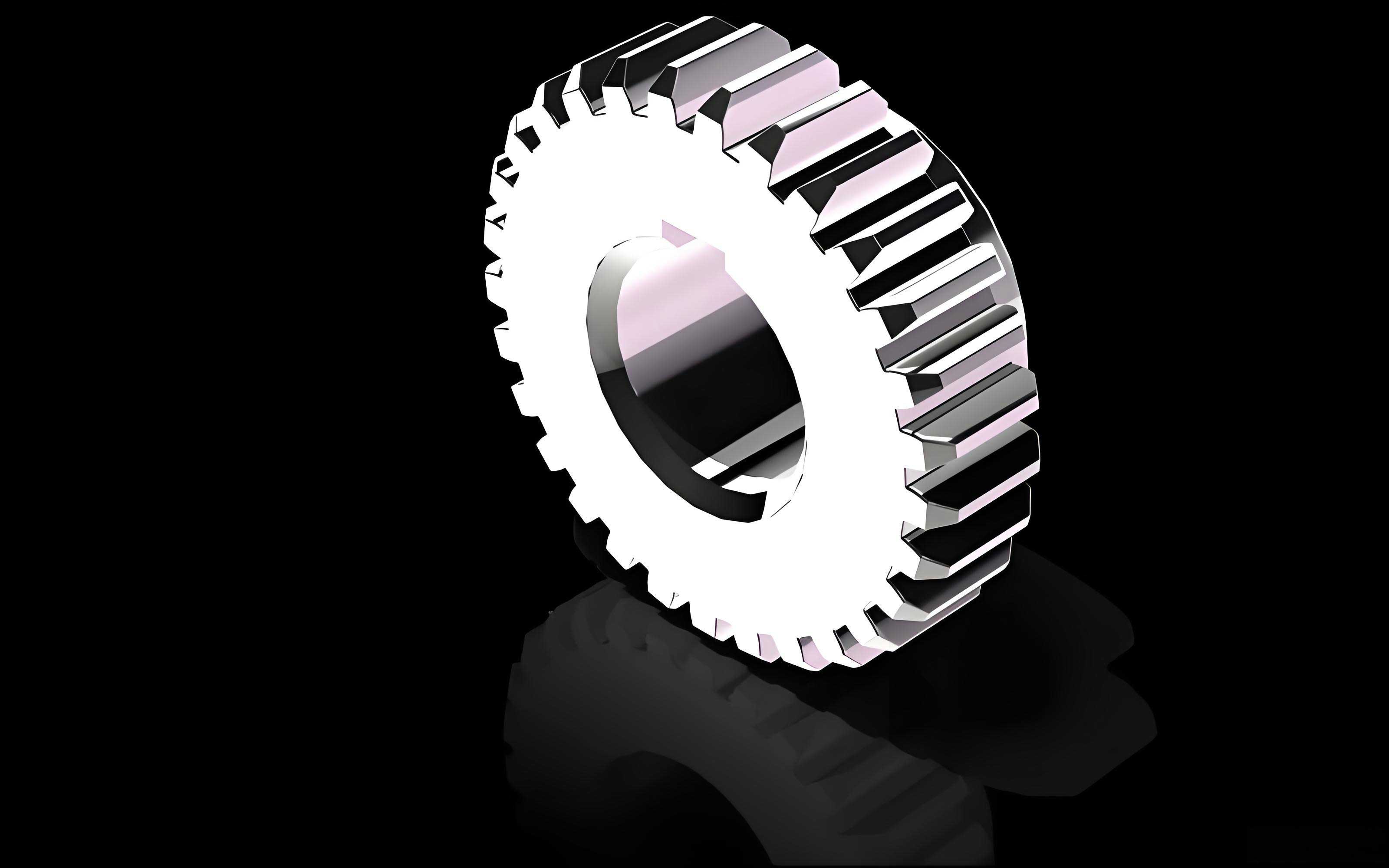
My research focuses on the nonlinear dynamic characterization of internal spur gear systems, with a particular emphasis on multi-state engagement and friction. Spur gears are fundamental components in numerous mechanical applications, and their dynamic behavior under varying operating conditions remains a critical area of study. The presence of backlash, time-varying mesh stiffness, and frictional forces introduces strong nonlinearities, leading to complex phenomena such as multi-state meshing, bifurcations, and chaos. This work aims to develop an accurate dynamic model of an involute internal spur gear pair, considering time-varying backlash, multi-state engagement, and the influence of lubrication and friction. I establish comprehensive formulations for dynamic mesh factors, including mesh force, mesh stiffness, damping, and friction coefficients, and then derive a dimensionless nonlinear dynamic model that captures five distinct meshing states: single-tooth drive-side, double-tooth drive-side, single-tooth back-side, double-tooth back-side, and tooth separation. Through extensive numerical simulations using Poincaré maps, bifurcation diagrams, Lyapunov exponents, and time-domain waveforms, I investigate the mechanisms of multi-state meshing and the influence of key parameters such as backlash, transmission error, meshing frequency, and load on the system’s global stability. Additionally, I propose a time-domain method for quantifying the proportion of dynamic instability cycles based on multi-state meshing, and I analyze the erosion of safe basins under parameter variations. The findings reveal that incomplete bifurcations and coexisting attractors significantly affect the system’s safe operation, and that the proper selection of parameters and initial conditions can enhance dynamic performance and prevent undesired behavior.
1. Dynamic Mesh Factor Modeling
Accurate calculation of dynamic mesh factors is the foundation for reliable gear system dynamics analysis. In this work, I propose improved models for the time-varying mesh force, mesh stiffness, mesh damping, and friction coefficient, explicitly incorporating the effects of tooth deformation, thermal expansion, nonlinear Hertzian contact, and multi-state lubrication.
1.1 Time-Varying Mesh Force
Based on the Johnson contact force model, I develop a modified mesh force formulation that includes energy dissipation. The normal mesh force between the gear teeth is expressed by:
$$ F_m = \frac{(a D(\tau)+b) L E^*}{D(\tau)} x^n \left[1 + \frac{3(1-c_e^2)}{4} \frac{\dot{x}}{\dot{x}^{(-)}}\right] $$
where \(D(\tau)\) is the time-varying backlash, \(L\) is the center distance, and \(E^* = E/[2(1-\mu^2)]\) is the composite Young’s modulus. The parameters \(a\), \(b\), and the exponent \(n\) depend on the magnitude of the backlash as detailed in the original work. This explicit force model is more efficient than traditional implicit formulations and remains valid for both small and large clearances.
1.2 Time-Varying Mesh Stiffness
The overall mesh stiffness \(k_m(t)\) is obtained by considering the contributions of elastic deformation, nonlinear Hertzian contact, and thermal deformation:
$$ \frac{1}{k_m(t)} = \frac{1}{k_e(t)} + \frac{1}{k_{eh}(t)} + \frac{1}{k_t(t)} $$
where \(k_e(t)\) is the elastic stiffness including bending, shear, axial compression, and fillet-foundation stiffness for both the pinion and the gear. The nonlinear Hertzian contact stiffness \(k_{eh}(t)\) is derived from \(k_{eh}=dF/d\sigma\), where \(\sigma\) is the total contact deformation, and it becomes zero when the teeth are separated. The thermal stiffness \(k_t(t)\) is introduced to account for tooth thermal deformation under operating temperatures, which is often neglected in conventional models.
Table 1 summarizes the components of the time-varying mesh stiffness model.
| Notation | Contribution | Main parameters |
|---|---|---|
| \(k_{eb}\) | Bending stiffness | Tooth geometry, Young’s modulus |
| \(k_{es}\) | Shear stiffness | Shear modulus, tooth cross-section |
| \(k_{ea}\) | Axial compression stiffness | Axial load component |
| \(k_{ef}\) | Fillet-foundation stiffness | Gear body geometry |
| \(k_{eh}\) | Nonlinear Hertzian contact stiffness | Instantaneous contact radius, force |
| \(k_t\) | Thermal stiffness | Temperature field, thermal expansion coefficient |
Numerical results indicate that including the nonlinear Hertzian and thermal stiffness reduces the overall mesh stiffness compared to the classical elastic-only model, which highlights the importance of these additional effects for accurate dynamic response prediction.
1.3 Time-Varying Mesh Damping
The mesh damping is related to the mesh stiffness and accounts for energy dissipation during impact and engagement. I adopt the impact damping model:
$$ c_m(t) = \frac{3(1-\psi)}{2\psi} \frac{k_m(t)}{\dot{x}^{(-)}} x^n $$
where \(\psi\) is the restitution coefficient (taken as 0.7). This formulation captures the energy loss that occurs during the switching between meshing states, which is crucial for realistic simulations.
1.4 Multi-State Lubrication Friction Coefficient
Friction at the tooth contact strongly affects the dynamic response. I introduce a friction coefficient model that switches between three lubrication regimes: elastohydrodynamic lubrication (EHL), mixed lubrication, and boundary lubrication. The regime is determined by the film parameter \(\Lambda(t) = h(t)/\sigma\), where \(h(t)\) is the minimum oil film thickness and \(\sigma\) is the combined surface roughness. The friction coefficient is given by:
$$ \mu(t) = \begin{cases}
\mu_E(t), & \Lambda(t) > 3.0 \\
\mu_M(t), & 1.0 \le \Lambda(t) \le 3.0 \\
\mu_C(t), & \Lambda(t) < 1.0
\end{cases} $$
The EHL friction is computed using a semi-empirical formula that accounts for slide-to-roll ratio, Hertzian pressure, and lubricant properties. The mixed lubrication friction is obtained from a full-film contact model, while the boundary regime uses a constant value typical of dry friction. This multi-state friction model enables a more realistic representation of the friction force variation along the line of action.
2. Multi-State Engagement Dynamics Model
Internal spur gear pairs exhibit different meshing states due to the combined effects of backlash and contact ratio. I classify the meshing states into five types based on the instantaneous relative displacement and the sign of the mesh force. These states are:
Figure 1 in the original work illustrates the drive-side and back-side lines of action for an internal spur gear pair. In my model, the dynamic mesh condition is determined by the relative displacement \(x = R_{bp}\theta_p – R_{bg}\theta_g – e(t)\), where \(R_{bp}\) and \(R_{bg}\) are the base circle radii of the pinion and gear, respectively, and \(e(t)\) is the transmission error excitation.
For a contact ratio between 1 and 2, the meshing cycle consists of alternating single- and double-tooth contact intervals. The time-varying backlash has different values in single and double-tooth regions due to the varying deformation at the contact point. I denote the half-backlash in the double-tooth region as \(D_d\) and that in the single-tooth region as \(D_s\), with \(D_s > D_d\). The boundary conditions for the five states are summarized in Table 2.
| Meshing state | Condition on relative displacement \(x\) | Condition on time interval |
|---|---|---|
| Double-tooth drive-side | \(x \ge D_d\) | \(mT_0 \le \tau \le (\varepsilon-1)mT_0\) |
| Single-tooth drive-side | \(x \ge D_s\) | \((\varepsilon-1)mT_0 \le \tau \le (m+1)T_0\) |
| Double-tooth back-side | \(x \le -D_d\) | \(mT_0 \le \tau \le (\varepsilon-1)mT_0\) |
| Single-tooth back-side | \(x \le -D_s\) | \((\varepsilon-1)mT_0 \le \tau \le (m+1)T_0\) |
| Tooth separation | \(|x| < D_d\) for all regions, and \(|x| < D_s\) in single-tooth interval | Any time |
Here \(T_0 = 2\pi/(z_p \omega_p)\) is the meshing period, and \(\varepsilon\) is the contact ratio. Using Newton’s second law for the torsional degrees of freedom, I derive the relative rotational equation of motion for each state:
Double-tooth drive-side:
$$ m_e \ddot{\bar{x}} + \left[1 + \mu_{d1}(\tau)g_{d1}(\tau)L_{d1}(\tau) + \mu_{d2}(\tau)g_{d2}(\tau)L_{d2}(\tau)\right] F_m = \bar{F}_m + \bar{F}_h(\tau) $$
Single-tooth drive-side:
$$ m_e \ddot{\bar{x}} + \left[1 + \mu_{d2}(\tau)g_{d2}(\tau)\right]F_m = \bar{F}_m + \bar{F}_h(\tau) $$
Double-tooth back-side:
$$ m_e \ddot{\bar{x}} – \left[1 + \mu_{b1}(\tau)g_{b1}(\tau)L_{b1}(\tau) + \mu_{b2}(\tau)g_{b2}(\tau)L_{b2}(\tau)\right]F_m = \bar{F}_m + \bar{F}_h(\tau) $$
Single-tooth back-side:
$$ m_e \ddot{\bar{x}} – \left[1 + \mu_{b2}(\tau)g_{b2}(\tau)\right]F_m = \bar{F}_m + \bar{F}_h(\tau) $$
Tooth separation:
$$ m_e \ddot{\bar{x}} = \bar{F}_m + \bar{F}_h(\tau) $$
Where \(m_e\) is the equivalent mass, \(\bar{F}_m\) is the external load term, \(\bar{F}_h(\tau)\) is the internal error excitation, and \(g\) and \(L\) are the effective friction arm and load sharing ratio, respectively. To unify these expressions, I introduce a state-dependent function \(h(\tau, \bar{x})\) and a mesh force function \(f(\bar{x}, \bar{D}(\tau))\). The resulting dimensionless equation is:
$$ \ddot{x} + h(t,x)\left[k(t)f(x,D(t)) + c(t)\dot{x}\right] = F + \xi \omega^2 \cos(\omega t) $$
where \(x = \bar{x}/D_c\), with \(D_c\) a characteristic length, and \(F\) is the dimensionless external force, \(\xi\) is the transmission error amplitude, and \(\omega\) is the dimensionless meshing frequency. The function \(h(t,x)\) takes different forms depending on whether the system is in single-tooth or double-tooth engagement, and also on whether the contact is on the drive-side or back-side. This dimensionless model is suitable for global nonlinear analysis.
3. Multi-State Meshing Mechanism and Nonlinear Dynamic Characteristics
3.1 Parameter Values and Poincaré Sections
I perform numerical simulations using the gear parameters listed in Table 3.
| Parameter | Pinion | Gear |
|---|---|---|
| Number of teeth | 30 | 70 |
| Module (mm) | 3 | 3 |
| Pressure angle (deg) | 20 | 20 |
| Face width (mm) | 25 | 25 |
| Young’s modulus (GPa) | 210 | 210 |
| Poisson’s ratio | 0.30 | 0.30 |
The dimensionless parameters are given in Table 4.
| Parameter | Symbol | Range |
|---|---|---|
| Meshing frequency | \(\omega\) | 0.01 – 3 |
| Load coefficient | \(F\) | 0.001 – 0.2 |
| Transmission error amplitude | \(\xi\) | 0.001 – 0.3 |
| Static backlash (half) | \(d_0\) | 0.30 – 2.00 |
To precisely identify the multi-state meshing behaviors, I define five Poincaré sections:
With these sections, each periodic motion can be labeled as \(n\)-\(p\)-\(q\)-\(r\)-\(s\), where \(n\) is the number of mesh cycles, and \(p,q,r,s\) are the numbers of crossings with each impact section during that period.
3.2 Mechanism of Tooth Separation and Back-Side Contact
To reveal the mechanism behind the multi-state meshing, I analyze the time histories of the dynamic mesh force and the relative displacement. It is found that the transition from drive-side contact to tooth separation occurs through a two-step process: first, the mesh force in the single-tooth region drops to zero and then reverses, but as long as the relative displacement remains larger than the single-tooth backlash, the contact continues. At the instant when \(x\) becomes equal to \(D_s\), a sudden jump to zero mesh force occurs, marking the onset of separation in the single-tooth region. Subsequently, the double-tooth region exhibits a similar behavior, and when \(x\) reaches \(D_d\), the entire mesh loses contact. This explains why the dynamic mesh force exhibits two abrupt changes when the system transitions from full drive-side contact to complete separation.
3.3 Influence of Backlash
I first examine the effect of the static backlash \(D\) on the system’s response. By increasing \(D\) while keeping \(\xi = 0.27\) and \(\omega = 1.4\), the bifurcation diagrams on the five Poincaré sections are obtained. For small \(D\), the system displays a stable 1-1-1-1-1 motion, implying one impact with each side within one period. As \(D\) increases, the motion undergoes a sequence of period-doubling bifurcations, leading to 2-1-1-1-1, 4-1-1-1-1, and then chaotic behavior. Further increase results in a crisis and the appearance of a period-3 window. Thereafter, chaos returns and eventually a long-period motion emerges. The overlapping of different Poincaré points indicates the coexistence of attractors. This study shows that larger backlash promotes richer nonlinear phenomena and increases the likelihood of tooth separation and back-side impacts.
3.4 Influence of Transmission Error
Next, I study the effect of the transmission error amplitude \(\xi\). With \(F=0.05\) and \(\omega=1.5\), the bifurcation diagram reveals an incomplete bifurcation at small \(\xi\): a period-1 motion coexists with a new period-2 motion, and the old solution remains stable. This coexistence persists over a wide range. As \(\xi\) grows, the system passes through a region of chaotic motion, then a periodic window of period-3, followed by a period-doubling cascade to chaos, and finally a stable period-3. The TLE spectrum confirms the chaotic regions. The results indicate that transmission error not only affects the vibration amplitude but also triggers the appearance of back-side contact and tooth separation, which are detrimental to gear durability.
3.5 Maximum Dynamic Mesh Force in Dual-Parameter Plane
To further illustrate the global effect of parameters, I calculate the maximum dynamic mesh force \(F_{\max}\) in the \((\xi, F)\) plane. The results show that when both \(\xi\) and \(F\) are small, \(F_{\max}\) exhibits a relatively smooth variation. As the parameters enter the chaotic regions, \(F_{\max}\) fluctuates sharply, indicating severe impact loads. The largest forces occur when both \(\xi\) and \(F\) are large, reaching a peak value of \(F_{\max}=1.340\). This analysis emphasizes that the maximum dynamic mesh force is highly sensitive to the multi-state meshing transformations.
4. Instability Characteristics and Global Stability
4.1 Detection of Multi-State Meshing
To characterize the dynamic instability, I introduce a Poincaré section \(\Pi_b\) for back-side contact and \(\Pi_s\) for tooth separation. The intersection of the phase trajectory with these sections indicates the occurrence of separation or back-side contact. Let \(\Gamma\) be the phase trajectory. If \(\Pi_s \cap \Gamma \ne \emptyset\) or \(\Pi_b \cap \Gamma \ne \emptyset\), then the system is considered to deviate from perfect meshing.
4.2 Dynamic Instability Cycle Proportion
I define a time-domain measure, the dynamic instability proportion \(P_{ID}\), which quantifies the fraction of time a gear system spends in unstable meshing states (tooth separation or back-side contact) during its steady-state response:
$$ P_{ID} = \frac{t_s + t_b}{t_d + t_s + t_b} $$
where \(t_d\) is the duration of drive-side contact, \(t_s\) is the duration of tooth separation, and \(t_b\) is the duration of back-side contact. These durations are computed by integrating the trajectory and recording the times when \(|x| \ge D\) (drive-side), \(|x| < D\) (separation), and \(x \le -D\) (back-side). This method provides a quantitative tool for evaluating the stability of a given dynamic solution.
4.3 Coexisting Attractors and Erosion of Safe Basins
Using a multi-initial bifurcation diagram, I investigate the global dynamics as a function of meshing frequency \(\omega\) and load \(F\). For example, with \(F=0.07\) and \(\xi=0.23\), as \(\omega\) increases from 0.1 to 3.0, the system exhibits multiple coexisting attractors. Table 5 summarizes the evolution of the attractors.
| \(\omega\) interval | Stable attractor | Unstable/coexisting attractor |
|---|---|---|
| 0.01 – 0.42 | 1-0-0-1-0 (healthy) | — |
| 0.42 – 0.54 | 1-0-0-1-0 | 1-1-1-1-1 (separation and back-side) |
| 0.54 – 0.58 | R1 (healthy) | 1-1-1-1-1 |
| 0.58 – 0.63 | R2 (unstable) | Q1 (unstable) |
| 0.63 – 0.72 | — | Q1 |
| 0.72 – 1.26 | — | Chaos |
| 1.26 – 1.52 | Q2 (stable) | P3 (unstable) |
| 1.80 – 1.89 | Q1 (stable) | P3 (unstable) |
| 1.89 – 2.30 | Q1 (stable) | P3 (unstable) |
| 2.30 – 3.00 | Q1 (stable) | — |
For instance, at \(\omega=0.42\), the system has two stable period-1 solutions, one with only drive-side and double-tooth separation (denoted \(P1\)) and one with all five states including back-side contact (denoted \(Q1\)). Their basins of attraction are shown in Figure 5.5(b). The healthy basin (for \(P1\)) occupies about 49% of the sampled region, while the unstable basin (for \(Q1\)) occupies 51%. As \(\omega\) increases, a period-doubling bifurcation causes \(R1\) to become period-2 and then chaotic, but \(Q1\) continues to exist. This incomplete bifurcation leads to the coexistence of a stable healthy solution and a chaotic solution, dramatically reducing the safe basin.
Similarly, when varying the load \(F\) with fixed \(\omega=1.4\) and \(\xi=0.09\), the system shows a reverse transition: at low load, chaos and high multi-stability are present; as \(F\) increases, the system settles into fewer coexisting attractors. Table 6 illustrates the changes.
| \(F\) interval | Healthy attractors | Unstable attractors |
|---|---|---|
| 0.0001 – 0.0021 | — | P3 and chaos |
| 0.0022 – 0.035 | — | P3 |
| 0.036 – 0.042 | — | P6 |
| 0.043 – 0.045 | — | P10 |
| 0.046 – 0.089 | — | Chaos |
| 0.09 – 0.104 | P2, Q4 | P3 |
| 0.105 – 0.117 | P2, Q2 | P3 |
| 0.118 – 0.2 | P1, Q2 | — |
At \(F=0.16\), the system displays two stable period motions: \(P1\) (1-1-0-1-0) and \(Q2\) (2-1-0-1-0), both free of back-side impacts. The basin of \(P1\) is about 78% of the sampled area, while \(Q2\) occupies 22%. As \(F\) is reduced, an incomplete bifurcation at \(G3\) introduces a period-3 unstable attractor \(R3\), and the basin of the healthy attractor shrinks. At \(F=0.104\), the unstable \(R3\) occupies 17%, while \(Q2\) and \(P2\) occupy 62% and 21%, respectively. Further decreasing \(F\) leads to a period-doubling of \(Q2\) into \(Q4\), and the unstable region grows to 58%. This erosion of the safe basin indicates that the system can become dangerously sensitive to initial conditions, especially under light loads.
4.4 Bifurcation and Safety Tree
To visualize the global evolution, I construct a bifurcation-safety tree, as shown in Figure 5.5. The tree uses different colored branches to represent healthy (stable) and unstable (unhealthy) periodic solutions. The occurrence of incomplete bifurcations is marked by the emergence of new branches from an existing branch that retains its stability. In this way, the tree clearly shows that global instability is often triggered by incomplete bifurcations, where a stable solution coexists with a newly generated unstable solution. The TLE spectrum corroborates the transition points where the Lyapunov exponent approaches zero.
5. Conclusion and Outlook
In this thesis, I have established a comprehensive dynamic model for an internal spur gear pair that accounts for time-varying backlash, multi-state meshing, and friction. The principal contributions are summarized as follows:
- I proposed improved dynamic mesh factor models that incorporate thermal stiffness and nonlinear Hertzian contact, leading to a more accurate mesh stiffness prediction.
- I classified the meshing states into five distinct regimes and derived a unified dimensionless nonlinear dynamic model that captures the switching behavior between them.
- I revealed the mechanisms of tooth separation and back-side contact by analyzing the abrupt changes in the dynamic mesh force.
- I investigated the effects of backlash, transmission error, meshing frequency, and load on the system’s bifurcation and chaos characteristics using multi-initial bifurcation diagrams and TLE spectra.
- I introduced a dynamic instability cycle proportion measure to quantify the time spent in unstable states, and I analyzed the erosion of safe basins due to coexisting attractors.
- I demonstrated that incomplete bifurcations are the main source of coexisting attractors, which may lead to severe sensitivity to initial conditions and reduced safety margins.
These findings provide valuable insights for the design of high-performance internal spur gear systems, enabling engineers to select appropriate parameters and initial conditions to avoid undesirable multi-state meshing and chaos. Future work would extend the model to include tooth profile modifications, wear, and three-dimensional dynamics, as well as experimental validation of the predicted phenomena.