
This article presents a comprehensive investigation into the contact stiffness and damping behavior of elastohydrodynamically lubricated (EHL) spur gear pairs. In this study, I developed analytical and numerical models to evaluate the normal contact stiffness, the oil film stiffness, and the oil film damping of a spur gear pair. The influence of operating conditions, surface roughness, starvation, and gear geometry parameters was systematically analyzed. The results provide insights into the dynamic response of lubricated gear contacts and support the development of more accurate gear dynamics models that include the lubricated tooth interface.
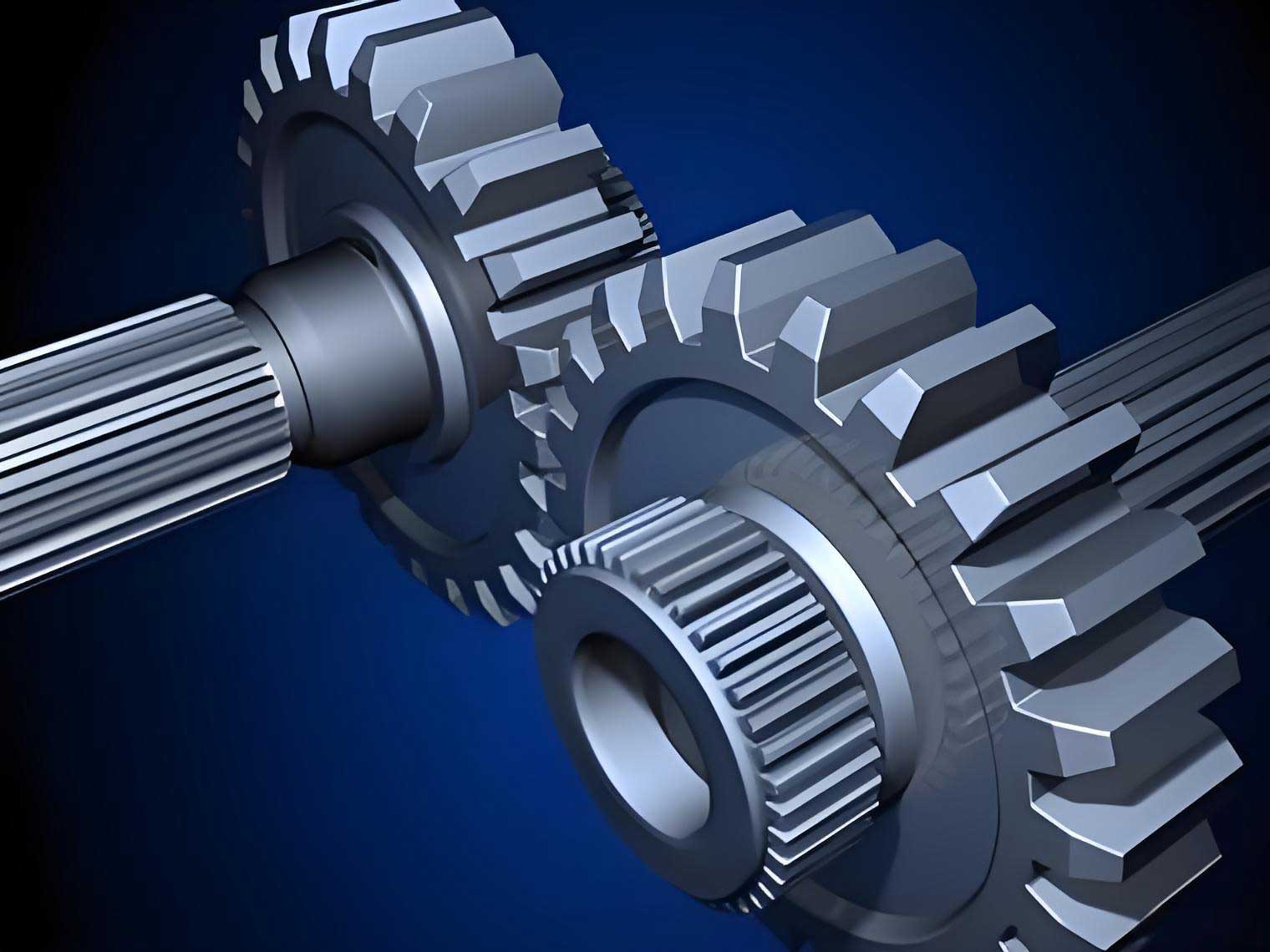
Spur gears are among the most widely used machine elements in power transmission systems. In practice, gear pairs operate under lubricated conditions, typically in the elastohydrodynamic lubrication (EHL) regime. Under load, both the gear tooth surfaces and the lubricating film deform elastically. The resulting stiffness of the tooth contact and of the oil film contributes to the overall mesh stiffness of the gear pair, which is a primary excitation source for gear vibration. In addition, due to the viscous nature of the lubricant, energy dissipation occurs inside the oil film when the film thickness varies dynamically, producing a damping effect. Although several studies have addressed the stiffness and damping of rolling bearings or lubricated point contacts, only a limited number of investigations have specifically considered the oil film stiffness and damping of a spur gear pair over a complete meshing cycle.
This paper aims to fill this gap by combining contact mechanics, elastohydrodynamic lubrication theory, and vibration theory. I first present the governing equations of line contact EHL and the numerical solution procedure. Then, I derive two analytical contact stiffness models based on the Hertz maximum deformation approach and the Yang–Sun linearized load-deformation relation. For the oil film stiffness, I propose four calculation methods, namely the minimum film thickness formula method, the central film thickness formula method, the global method, and the average film thickness method. Next, I develop two numerical approaches to quantify the oil film damping: the harmonic excitation method and the free vibration energy method. Finally, the proposed models are applied to a FZG type spur gear pair to investigate the variations of contact stiffness, oil film stiffness, and oil film damping along the line of action under different torque, speed, and gear modification conditions.
1. Elastohydrodynamic Lubrication Model
The lubricated contact between a pair of spur gear teeth can be modeled as a two-dimensional line contact between two elastic cylinders. The classical EHL model consists of the Reynolds equation, the film thickness equation, the viscosity–pressure relationship, the density–pressure relationship, and the load balance equation. For an incompressible Newtonian fluid under steady-state conditions, the one-dimensional Reynolds equation is
$$
\frac{\partial}{\partial x}\left(\frac{\rho h^3}{12\eta}\frac{\partial p}{\partial x}\right) – u_r \frac{\partial (\rho h)}{\partial x} – \frac{\partial (\rho h)}{\partial t} = 0,
$$
where \(x\) is the coordinate along the rolling direction, \(\rho\) is the lubricant density, \(h\) is the local film thickness, \(\eta\) is the dynamic viscosity, \(p\) is the hydrodynamic pressure, \(u_r=(u_1+u_2)/2\) is the rolling velocity, and \(t\) is time. When the transient term is omitted, the steady-state Reynolds equation is recovered.
The film thickness between two smooth elastic bodies is expressed as
$$
h(x,t) = h_0(t) + \frac{x^2}{2R} – \frac{2}{\pi E’} \int_{-\infty}^{+\infty} \ln|x-x’|\, p(x’,t)\, dx’,
$$
where \(h_0\) is the rigid body displacement, \(R\) is the equivalent radius of curvature, and \(E’\) is the equivalent elastic modulus given by
$$
\frac{1}{E’} = \frac{1}{2}\left( \frac{1-\nu_1^2}{E_1} + \frac{1-\nu_2^2}{E_2} \right).
$$
The Dowson–Higginson density–pressure relationship is used:
$$
\rho(p) = \rho_0 \frac{0.59\times10^9 + 1.34 p}{0.59\times10^9 + p},
$$
and the Roelands viscosity–pressure equation is adopted:
$$
\eta(p) = \eta_0 \exp\left\{ \left(\ln\eta_0 + 9.67\right) \left[ \left(1+\frac{p}{p_0}\right)^z – 1 \right] \right\},
$$
where \(p_0 = 5.1\times10^9\,\mathrm{Pa}\) and \(z=0.68\). The load balance equation is
$$
F(t) = B \int_{-\infty}^{+\infty} p(x,t)\, dx,
$$
where \(F\) is the line load and \(B\) is the contact length.
To solve the EHL equations numerically, I used the dimensionless Hertzian variables
$$
X = \frac{x}{b}, \quad P = \frac{p}{p_H}, \quad H = \frac{h R}{b^2}, \quad T = \frac{t u_r}{b},
$$
where \(b\) is the Hertzian half-width
$$
b = \sqrt{\frac{8 F R}{\pi B E’}},
$$
and \(p_H\) is the maximum Hertzian pressure
$$
p_H = \frac{2 F}{\pi b B}.
$$
The dimensionless Reynolds equation becomes
$$
\frac{\partial}{\partial X}\left(\varepsilon \frac{\partial P}{\partial X}\right) – \frac{\partial (\bar{\rho} H)}{\partial X} – \frac{\partial (\bar{\rho} H)}{\partial T} = 0,
$$
with
$$
\varepsilon = \frac{\bar{\rho} H^3}{\bar{\eta} \lambda},\qquad \lambda = \frac{12 \eta_0 u_r R^2}{b^3 p_H}.
$$
I used a mixed relaxation scheme that combines the Gauss–Seidel method for regions where \(\varepsilon/\Delta X^2\) is large and the Jacobi distributive method where it is small. The computational domain was chosen as \(X \in [-5, 1.5]\) and 2048 mesh points were found to be sufficient to achieve grid-independent results. The numerical model was validated by comparing the minimum and central film thickness values with the Dowson–Higginson empirical formulas. Table shows the model parameters used in the numerical simulations.
| Parameter | Symbol | Value |
|---|---|---|
| Ambient viscosity | \(\eta_0\) | 0.04 Pa s |
| Pressure-viscosity coefficient | \(\alpha_l\) | 2.2e-8 Pa⁻¹ |
| Elastic modulus | \(E_1, E_2\) | 2.0e11 Pa |
| Poisson ratio | \(\nu_1, \nu_2\) | 0.3 |
| Contact density | \(\rho_c\) | 7850 kg/m³ |
| Equivalent radius | \(R\) | 0.01–0.05 m |
2. Contact Stiffness Models
The deformation of the gear tooth surfaces under load gives rise to a normal contact stiffness. Two analytical models were considered in this work: the Hertzian model and the Yang–Sun linearized model.
For a line contact, the Hertzian maximum elastic deformation is
$$
\delta_{\max} = R – \sqrt{R^2 – b^2}.
$$
Since \(b^2 = 2R\delta_{\max} – \delta_{\max}^2\), the relation between the total normal load \(f = F B\) and the deformation can be written as
$$
f = \frac{\pi B E’}{4 R} \left( \delta_{\max}^2 – \frac{\delta_{\max}^2}{2R} \right)?
$$
I derived the more accurate expression:
$$
f = \frac{\pi E’ B}{8 R} \left(2R\delta_{\max} – \delta_{\max}^2\right).
$$
Differentiating with respect to the deformation yields the Hertz contact stiffness:
$$
k_{c,\mathrm{Hertz}} = \frac{df}{d\delta_{\max}} = \frac{\pi B E’}{4}\left(1-\frac{\delta_{\max}}{R}\right).
$$
This expression clearly shows that the Hertzian contact stiffness depends on the deformation and therefore slightly on the applied load, because \(\delta_{\max}/R\) varies with load. However, for typical gear contacts this ratio is small, so the load dependence is weak.
In contrast, Yang and Sun proposed a linearized load–deformation relation:
$$
f = \frac{\pi B E’}{4} \delta_{\max},
$$
which leads to a constant contact stiffness:
$$
k_{c,\mathrm{YS}} = \frac{\pi B E’}{4}.
$$
This linearized model is convenient for gear dynamics analyses because it is independent of the load and deformation. In my study, I compared the two models over a wide range of loads (\(F\) from \(2.5\times10^5\) to \(6.25\times10^5\,\mathrm{N/m}\)) and equivalent radii (\(R\) from 0.01 to 0.1 m). The magnitude of the Yang–Sun stiffness was of the same order as the Hertzian stiffness, confirming that the linearized load–deformation relation is reasonable.
3. Oil Film Stiffness Calculation Methods
The lubricating film between the gear teeth also deforms under load, and this deformation defines an oil film stiffness. I proposed four methods to compute the oil film stiffness from the EHL solution.
3.1 Empirical formula methods
The Dowson–Higginson minimum film thickness formula is
$$
h_m = 2.65 \frac{U^{0.7} G^{0.54} R}{W^{0.13}},
$$
where \(U = \eta_0 u_r / (E’ R)\), \(G = \alpha_l E’\), and \(W = F / (E’ R)\). Since \(h_m \propto F^{-0.13}\), the oil film stiffness based on the minimum film thickness can be obtained by differentiating \(F\) with respect to \(h_m\):
$$
k_{hm} = \frac{dF}{dh_m} = \frac{F}{0.13 h_m}.
$$
Similarly, the Dowson–Higginson central film thickness formula is
$$
h_c = 3.06 \frac{U^{0.69} G^{0.56} R}{W^{0.10}},
$$
and the corresponding central film stiffness is
$$
k_{hc} = \frac{dF}{dh_c} = \frac{F}{0.10 h_c}.
$$
These empirical formulas are valid only for smooth surfaces and fully flooded conditions, so I coupled them with the numerical EHL solver for more general cases.
3.2 Global numerical method
In the global method, the contact region is divided into small spring elements in parallel. At each node \(i\), the stiffness contribution is \(\Delta f_i / \Delta h_i\), where \(\Delta f_i = B p_i \Delta x\) is the local load increment and \(\Delta h_i\) is the local film thickness change due to a small load change. The total oil film stiffness is the sum of all local contributions:
$$
k_{\mathrm{glo}} = \sum_{i=n_1}^{n_2} \frac{\Delta f_i}{\Delta h_i},
$$
where \(n_1\) and \(n_2\) denote the inlet and outlet boundaries of the pressurized region. This method captures the complete pressure and film thickness distributions and is therefore considered the most detailed numerical approach.
3.3 Average film thickness method
A simpler numerical method uses the average film thickness over the contact region. The oil film stiffness is defined as
$$
k_{\mathrm{ave}} = \frac{\Delta F}{\Delta \bar{h}},
$$
where \(\Delta F\) is the total load increment and \(\Delta \bar{h}\) is the change of the average film thickness between the upstream and downstream boundaries of the pressurized region. This method is computationally efficient and was found to give results consistent with the global method for most operating conditions.
In order to determine a suitable load perturbation, I examined the effect of the load increment ratio \(\Delta F / F\) on the oil film stiffness at four extreme cases (heavy load–low speed, light load–low speed, heavy load–high speed, and light load–high speed). The results showed that the oil film stiffness is nearly insensitive to \(\Delta F / F\) in the range from 0.005 to 0.05. Therefore, I selected \(\Delta F / F = 0.0125\) for subsequent simulations.
4. Influence of Operating Conditions on Oil Film Stiffness
Using the numerical EHL model, I studied how the oil film stiffness varies with load and rolling speed. The Moes parameters \(M\) and \(L\) were used to characterize the operating conditions:
$$
M = \frac{F}{\eta_0 u_r R} \left( \frac{\eta_0 u_r}{E’ R} \right)^{-1/2}, \qquad L = \alpha_l E’ \left( \frac{\eta_0 u_r}{E’ R} \right)^{1/4}.
$$
Figure shows the minimum film thickness values predicted by the numerical model and the Dowson–Higginson formula for a range of loads from \(1\times10^5\) to \(2\times10^6\,\mathrm{N/m}\) and rolling speeds from 0.1 to 10 m/s. The numerical model matched the empirical formula closely.
The oil film stiffness obtained with the four methods is shown in Figure as a function of load and rolling speed. All four methods predicted the same qualitative trends: the oil film stiffness increases with increasing load and decreases with increasing rolling speed. Physically, a higher load compresses the film and makes it more difficult to deform further, while a higher rolling speed generates a thicker film and thus reduces the stiffness. In the heavy-load, low-speed region, the global method and the Dowson–Higginson minimum film formula gave somewhat larger stiffness values than the other two methods, but overall the differences were moderate. At a given load, the oil film stiffness was generally two to three orders of magnitude higher than the Hertzian contact stiffness, as shown in the comparison figure.
| Case | Load \(F\) (N/m) | Speed \(u_r\) (m/s) | \(k_{\mathrm{ave}}\) (N/m) | \(k_{c,\mathrm{Hertz}}\) (N/m) |
|---|---|---|---|---|
| Light load, low speed | 1e5 | 0.1 | ~3e11 | ~1.7e9 |
| Heavy load, low speed | 1e6 | 0.1 | ~1.2e12 | ~1.7e9 |
| Light load, high speed | 1e5 | 10 | ~1e11 | ~1.7e9 |
| Heavy load, high speed | 1e6 | 10 | ~4e11 | ~1.7e9 |
5. Surface Roughness and Starvation Effects
Real gear surfaces are rough. In this study, I modeled the surface roughness as a sinusoidal waviness superimposed on the smooth film thickness equation:
$$
r_r(x) = a \cos\left(\frac{2\pi x}{\lambda_b}\right),
$$
where \(a\) is the roughness amplitude and \(\lambda_b\) is the wavelength. The dimensionless roughness amplitude is defined as \(A_{mp} = a / R\) in the dimensionless formulation. I investigated the effect of roughness amplitude and wavelength on the pressure distribution, film thickness, and oil film stiffness. The results indicate that the oil film stiffness decreases slightly when the roughness amplitude increases, because a larger amplitude increases the average film thickness and thus reduces the resistance to compression. For a fixed amplitude, an increase in the wavelength leads to a higher oil film stiffness, and the influence of the amplitude becomes less pronounced at longer wavelengths.
Starvation is another important factor in gear lubrication. To simulate starved conditions, I used the Elrod algorithm with a partial film thickness parameter \(\theta(X)\), which represents the ratio between the actual film thickness and the clearance. The inlet oil film thickness \(H_{oil}\) controls the amount of oil supplied to the contact. Figure shows the pressure and film thickness distributions for different inlet oil supply levels. As \(H_{oil}\) increases, the pressure profile approaches the fully flooded solution and the film thickness increases. For low rolling speeds, the oil film stiffness first increases with increasing \(H_{oil}\) and then levels off. For high rolling speeds, the stiffness decreases with increasing \(H_{oil}\). This non-monotonic behavior arises from the competing effects of the inlet supply on the pressurized region and the overall film level.
| Rolling speed \(u_r\) | Inlet oil supply \(H_{oil}\) | Trend of \(k_{oil}\) with \(H_{oil}\) |
|---|---|---|
| 0.1 m/s | 0.1–1.0 | Increase then stabilize |
| 1 m/s | 0.1–1.0 | Increase then stabilize |
| 10 m/s | 0.1–1.0 | Decrease |
6. Oil Film Damping Calculation
The oil film damping arises from the viscous dissipation in the lubricant film when the film thickness changes dynamically. I developed two numerical approaches to quantify this damping: the harmonic excitation method and the free vibration energy method.
6.1 Harmonic excitation method
In this method, a sinusoidal load is applied to the EHL contact:
$$
f(t) = f_0 + f_a \sin(\omega t),
$$
where \(f_0\) is the mean load and \(f_a\) is the load amplitude. The equation of motion of the contact system is
$$
\frac{m_c}{B} \frac{d^2 h_0}{dt^2} + \int p(x,t)\, dx = f(t),
$$
where \(m_c\) is the equivalent mass of the contact bodies. In dimensionless form, the load equation becomes
$$
\frac{2}{M_c}\frac{d^2 H_0}{dT^2} + \int P(X,T)\, dX = 1 + A_f \sin(\Omega_e T),
$$
with \(M_c = m_c u_r^2 / (f_0 R B)\) and \(\Omega_e = \omega b/u_r\). For a harmonic response
$$
H_0(T) = A_1 \cos(\Omega_e T),
$$
the damping force per unit length is modeled as
$$
W_C(T) = D \frac{dH_0}{dT},
$$
where \(D\) is the dimensionless damping coefficient. The area enclosed by the hysteresis loop of \(H_0\) versus the imposed load gives the energy dissipated per cycle:
$$
E_C = \int_0^{T_{period}} W_C \frac{dH_0}{dT}\, dT = – \pi D A_1^2 \Omega_e.
$$
By evaluating the loop area numerically, I obtained the dimensionless damping coefficient \(D\) and then the physical damping coefficient:
$$
c_{\mathrm{har}} = \frac{D f_0 R}{B b u_r}.
$$
I studied the influence of the excitation frequency and amplitude on the damping. The results showed that \(c_{\mathrm{har}}\) is nearly independent of the frequency and amplitude over a wide range, so the oil film damping can be considered as a purely viscous damping coefficient.
6.2 Free vibration energy method
In the free vibration method, the system is released from an initial perturbation away from the equilibrium position. The equation of motion is
$$
m_c \frac{d^2 h_0}{dt^2} + c_{\mathrm{free}} \frac{d h_0}{dt} + k_o h_0 = f_0,
$$
where \(k_o\) is the oil film stiffness in the equilibrium state. Defining \(\Delta h_0(t) = h_0(t) – h_0(\infty)\), I multiplied the equation by \(\Delta \dot{h}_0\) and integrated over time. Using the energy conservation principle, the total initial elastic energy equals the energy dissipated by the damper:
$$
\frac{1}{2} k_o [\Delta h_0(0)]^2 = c_{\mathrm{free}} \int_0^\infty [\Delta \dot{h}_0(t)]^2 dt.
$$
Thus, the free vibration damping coefficient is
$$
c_{\mathrm{free}} = \frac{k_o [\Delta h_0(0)]^2}{2 \int_0^\infty [\Delta \dot{h}_0(t)]^2 dt}.
$$
I also computed the damping ratio and the logarithmic decrement from the time response:
$$
\zeta = \sqrt{1 – \left(\frac{\omega_d}{\omega_n}\right)^2}, \qquad \delta = \frac{2\pi\zeta}{\sqrt{1-\zeta^2}},
$$
where \(\omega_n\) is the undamped natural frequency and \(\omega_d\) is the damped natural frequency. The undamped frequency was obtained from a dry contact model, while the damped frequency was extracted from the free vibration response of the EHL contact.
6.3 Effect of operating conditions on oil film damping
Using both methods, I evaluated the oil film damping for different loads and rolling speeds. Figure shows the variation of \(c_{\mathrm{har}}\) and \(c_{\mathrm{free}}\) with load for a rolling speed of 3 m/s. Both methods indicate that the oil film damping decreases as the load increases. This is because the higher load increases the viscosity through the pressure–viscosity effect, which reduces the ability of the film to dissipate energy. The damping ratio, on the other hand, increases with load, meaning that the amplitude decay is faster at higher loads.
Figure shows the effect of rolling speed on the damping. As the rolling speed increases, the oil film thickness increases and the damping coefficient decreases. The damping ratio and logarithmic decrement also decrease with increasing speed, indicating that the film is less effective in suppressing vibrations at high speeds. The harmonic excitation method generally yielded slightly larger damping values than the free vibration method, but the trends were consistent.
| Load \(f_0\) (N) | Speed \(u_r\) (m/s) | \(c_{\mathrm{har}}\) (N s/m) | \(c_{\mathrm{free}}\) (N s/m) |
|---|---|---|---|
| 5000 | 3 | ~1.2e7 | ~8.0e6 |
| 9000 | 3 | ~6.0e6 | ~4.0e6 |
| 7000 | 1 | ~2.5e7 | ~1.8e7 |
| 7000 | 10 | ~5.0e6 | ~3.0e6 |
7. Application to a FZG Spur Gear Pair
To investigate the practical behavior of a spur gear pair, I considered the FZG type A and type C test gears. The gear geometry parameters are listed in the table below.
| Parameter | Type A | Type C |
|---|---|---|
| Gear ratio \(i\) | 1.5 | 1.5 |
| Module \(m\) (mm) | 4.5 | 4.5 |
| Number of teeth \(z_1, z_2\) | 16, 24 | 16, 24 |
| Addendum coefficient \(h_a^*\) | 1.0 | 1.0 |
| Pressure angle \(\alpha_0\) | 20° | 20° |
| Face width \(B\) (m) | 0.01 | 0.01 |
| Profile shift \(x_1\) | 0.8532 | 0.1817 |
| Profile shift \(x_2\) | −0.5 | −0.1715 |
For a spur gear pair, the normal load along the line of action (LOA) is not constant. During double-tooth contact, the load is shared by two tooth pairs, whereas during single-tooth contact the entire load is carried by one pair. I used a simplified piecewise load distribution: the load varies linearly in the double-tooth regions and remains equal to the total load in the single-tooth region. The equivalent radius and rolling speed also vary along the LOA. These variations were computed from the gear geometry:
$$
R_1 = R_{p1}\sin\alpha’ + \zeta, \qquad R_2 = R_{p2}\sin\alpha’ – \zeta,
$$
where \(R_{p1}\) and \(R_{p2}\) are the pitch circle radii, \(\alpha’\) is the operating pressure angle, and \(\zeta\) is the distance from the pitch point. The equivalent radius is
$$
R = \frac{R_1 R_2}{R_1 + R_2}.
$$
The rolling and sliding velocities at the contact point are
$$
u_1 = \omega_1 R_1, \quad u_2 = \omega_2 R_2, \quad u_r = \frac{u_1+u_2}{2}, \quad u_s = u_1-u_2.
$$
8. Results for the Spur Gear Pair
8.1 Contact stiffness of the gear pair
Using the gear geometry and the load distribution for \(T_1 = 300\,\mathrm{N\,m}\) and \(n_1 = 1000\,\mathrm{r/min}\), I computed the Hertzian maximum deformation and the contact stiffness along the LOA. The maximum deformation follows the load distribution, being smallest in the double-tooth regions and largest in the single-tooth region. The contact stiffness is slightly higher at the beginning of engagement and lower at the highest point of single-tooth contact. The contact stiffness is almost independent of the input speed, because the deformation is governed by the quasi-static load and geometry. When the input torque is increased, the deformation increases and the contact stiffness decreases slightly.
8.2 Oil film stiffness of the gear pair
Figure shows the minimum film thickness along the LOA for the type A gear at \(T_1 = 300\,\mathrm{N\,m}\) and \(n_1 = 1000\,\mathrm{r/min}\). The minimum film thickness is lower in the single-tooth region, especially at the lowest and highest points of single-tooth contact. The four oil film stiffness methods give similar distributions along the LOA. The stiffness in the single-tooth region is higher than in the double-tooth region, because the higher load compresses the film. At the transition points between single and double tooth contact, the oil film stiffness exhibits a jump due to the sudden load change.
I also studied the effect of input torque and speed on the oil film stiffness. As the input torque increases, the oil film stiffness increases at every position along the LOA. As the input speed increases, the oil film thickness increases and the oil film stiffness decreases. These trends are consistent with the results from the line contact model.
8.3 Oil film damping of the gear pair
Using the harmonic excitation method, I evaluated the oil film damping along the LOA for the type A gear under the same operating condition. The damping is lower in the single-tooth region and higher in the double-tooth region. This suggests that the viscous dissipation is more effective when the load is shared by two tooth pairs. An increase in input torque reduces the damping, and an increase in input speed also reduces the damping. The Ankouni fitting formula, which expresses the dimensionless damping as
$$
D = \frac{4.3 (L M)^{1.2}}{1 + 3 (L M)^{0.85}},
$$
was also evaluated along the LOA and showed the same dependency on torque and speed.
8.4 Effect of profile shift
The FZG type C gear has different profile shift coefficients compared to type A. This changes the positions of the single-tooth contact region, the length of the line of action, and the local radii and velocities. I compared the type A and type C gears under identical load and speed conditions. The results show that the type C gear has a slightly longer line of action and a smaller equivalent radius at the same normalized position. Consequently, the minimum film thickness of the type C gear is lower, and both the oil film stiffness and the oil film damping are lower than those of the type A gear. This demonstrates that the profile shift, by altering the contact geometry and kinematics, has a significant influence on the lubricated contact dynamics of a spur gear pair.
| Gear type | LOA length | Minimum film thickness at single contact | Oil film stiffness (average) | Oil film damping (average) |
|---|---|---|---|---|
| Type A | Base | Higher | Higher | Higher |
| Type C | Longer | Lower | Lower | Lower |
9. Conclusions
In this study, I developed a comprehensive numerical framework to investigate the contact stiffness, oil film stiffness, and oil film damping of elastohydrodynamically lubricated spur gear pairs. The main conclusions are summarized as follows:
- The Hertzian contact stiffness depends weakly on the load, while the Yang–Sun linearized model provides a constant contact stiffness of the same order of magnitude. The linearized load–deformation relation is therefore reasonable for gear dynamics applications.
- Four oil film stiffness methods, namely the minimum film thickness formula, the central film thickness formula, the global method, and the average film thickness method, give consistent results over a wide range of loads and speeds. The oil film stiffness increases with increasing load and decreases with increasing rolling speed. Under the same conditions, the oil film stiffness is two to three orders of magnitude higher than the contact stiffness.
- Surface roughness with larger amplitude reduces the oil film stiffness, while a larger wavelength increases it. Starved lubrication affects the stiffness in a non-monotonic manner that depends on the rolling speed.
- The oil film damping can be quantified by the harmonic excitation method and the free vibration energy method. Both methods show that the damping decreases with increasing load and rolling speed. The harmonic method gives slightly higher values than the free vibration method.
- For the FZG spur gear pair, the contact stiffness varies along the LOA and is mostly influenced by the load distribution. The oil film stiffness and damping also vary along the LOA, with lower damping in the single-tooth region. Increasing input torque increases oil film stiffness but decreases damping; increasing input speed decreases both stiffness and damping.
- Profile shift modifies the contact geometry and kinematics, leading to noticeable changes in the oil film stiffness and damping of the spur gear pair.
The proposed models provide a solid basis for incorporating the lubricated tooth interface characteristics into gear system dynamics, which is essential for accurate prediction of vibration and noise in modern gear drives.