
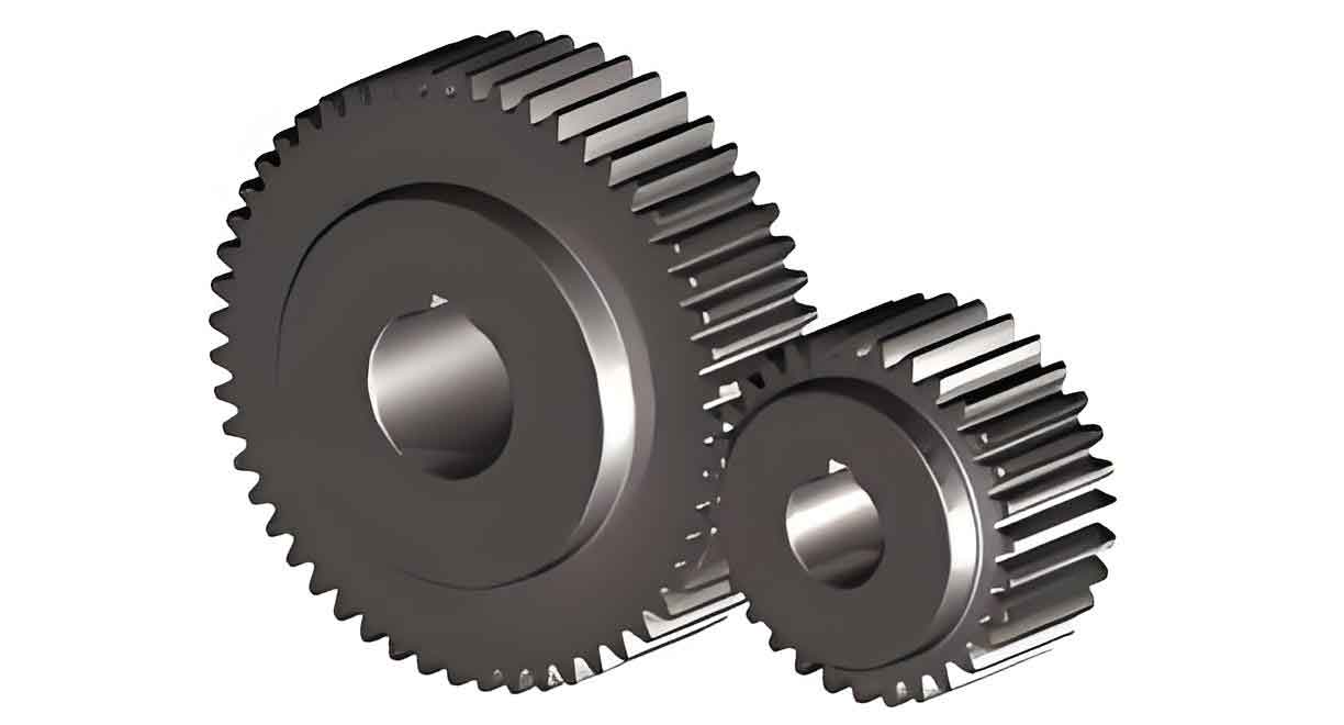
Gear transmission systems serve as core power transmission components in modern industrial equipment, and their transmission stability and fatigue resistance directly affect operational reliability, transmission efficiency, and running smoothness. Single-stage spur gears are widely used in critical applications such as traction system gearboxes of high-speed trains, reducer gear sets, and couplings, due to their simple structure and high transmission efficiency. However, under high speed, heavy load, and complex operating conditions, the gear meshing contact area is prone to severe vibration, noise, tooth surface pitting, tooth surface bonding, and other fatigue failures caused by insufficient lubrication. The nonlinear dynamic characteristics of spur gear systems under different lubrication states have not been fully revealed. In this study, a single-stage spur gear with lubrication in one degree of freedom is taken as the research object, and the interaction between lubrication characteristics and nonlinear dynamics is systematically investigated through theoretical modeling, numerical simulation, and continuation shooting method.
Introduction
With the rapid advancement of China’s railway industry, passenger and freight vehicle technologies are constantly being updated, and running speeds continue to increase. The CR450 high-speed train, currently the fastest in China, can reach test speeds of 450 km/h with an operating speed of 400 km/h. The gearbox is the core component driving high-speed operation of the CR450 multiple unit. Under such high-speed working conditions, the gear sustained speed must remain at 3000–4000 rpm, and the operating temperature range is between −40°C and 120°C. Under such long-term high-temperature and high-pressure conditions, gear transmission systems require extreme-pressure additive lubricating oil to avoid tooth surface gluing or tooth surface pitting, thereby extending gear service life. Gear lubrication is crucial, but vibration problems caused by insufficient gear lubrication are equally non-negligible, which greatly affects the stability of gear transmission systems. In recent years, scholars at home and abroad have conducted extensive research on gear vibration based on elastohydrodynamic lubrication (EHL) theory.
In exploring the dynamics of gear systems, many scholars have established gear dynamic models including dry friction or lubrication. Through numerical simulation based on theoretical analysis, they have conducted in-depth investigations on nonlinear factors affecting gear characteristics, such as gear time-varying stiffness, backlash, and static comprehensive transmission error. These factors can not only avoid vibration generated during gear operation but also provide instructive suggestions for gear system design and optimization. When studying gear system dynamics and stability under lubricated conditions, it is necessary to mention the phenomenon of attractor coexistence in gear transmission systems. The coexistence of these attractors and their complex transition and evolution laws have strong correlation with gear system stability. Under the mutual transition influence of these stable and unstable attractors, the gear system will also produce varying degrees of vibration, leading to unstable macroscopic gear power transmission.
This study simulates the lubrication characteristics of spur gear systems, reveals the distribution characteristics of lubricating oil film pressure field and geometric morphology, constructs a dynamic mathematical stiffness model of the oil film, and then couples it with gear contact stiffness to obtain the combined stiffness simulation curve. This provides theoretical support for subsequent nonlinear vibration response and dynamic behavior analysis of spur gears. Through multi-initial bifurcation diagrams, continuation shooting method, Floquet multiplier theory, and maximum Lyapunov exponent, the transition laws and bifurcation phenomena of coexisting attractors are investigated for the lubricated spur gear system. Phase diagrams, Poincaré maps, and attraction domains are used to study the stability of coexisting attractors, revealing the influence of nonlinear characteristics under different lubrication states on system dynamics.
Elastohydrodynamic Lubrication Theory for Line Contact
Many contact problems such as spur gears and cylindrical roller bearings can be assumed to be half-infinite body line contact problems. These complex mechanical problems can be conceptually simplified to the interaction between an elastic structure with an equivalent radius and a rigid plane. Due to the pressure-viscosity relationship of the lubricant, the oil film exists in the nominal contact area, which inhibits the motion between these contact bodies.
The line contact EHL model is established with the following conditions: in the dimensionless model, only oil film pressure needs to be considered, and gravity effects are removed; the oil film thickness between contacting component surfaces under external load reaches only micrometer order under normal conditions; the viscosity and density of the oil film along the normal load direction do not change; during component motion, the lubricant remains relatively stationary with the contact surface, meaning the contact body velocity can approximate the lubricant flow velocity.
The model transforms the lubricant into an equivalent elastic cylinder interacting with a rigid plane. Under normal load, the equivalent elastic cylinder moves toward the rigid plane. Due to the pressure-viscosity relationship of the lubricant, the oil film is compressed and produces compressive deformation in the contact area. The line contact EHL model is established based on this simplified theory.
The Five Basic Equations of EHL
One-dimensional line contact Reynolds equation:
$$\frac{\partial}{\partial x}\left(\varepsilon \frac{\partial p}{\partial x}\right) = \frac{\partial(\rho h)}{\partial x}$$
where $p$ is the lubricant film pressure, $h$ is the film thickness, $\eta$ is the lubricant viscosity, $\rho$ is the lubricant density, and:
$$\varepsilon = \frac{\rho h^{3}}{12\eta \lambda}, \quad \lambda = \frac{6\eta_{0} U_{\mathrm{s}}}{b p_{\mathrm{H}}}$$
The film thickness equation is:
$$h(x) = h_{0} + \frac{x^{2}}{2R} – \frac{2}{\pi E’}\int_{x_{\mathrm{in}}}^{x_{\mathrm{out}}} p(x’)\ln(x-x’)^{2} \, dx’$$
where $h_0$ is the geometric gap of the contacting bodies, $R$ is the equivalent radius of curvature, $E’$ is the equivalent elastic modulus of the two contacting bodies:
$$\frac{1}{E’} = \frac{1}{2}\left(\frac{1-\nu_{1}^{2}}{E_{1}} + \frac{1-\nu_{2}^{2}}{E_{2}}\right)$$
The pressure boundary conditions are:
$$p(x_{\mathrm{in}}) = p(x_{\mathrm{out}}) = 0, \quad p(x) \geq 0$$
The viscosity-pressure equation is:
$$\eta = \eta_{0} \exp\left\{\left[\ln(\eta_{0}) + 9.67\right]\left[(1 + 5.1 \times 10^{-9}p)^{z} – 1\right]\right\}$$
where:
$$z = \frac{\alpha}{5.1 \times 10^{-9}\left[\ln(\eta_{0}) + 9.67\right]}$$
The density-pressure equation is:
$$\rho = \rho_{0}\left(1 + \frac{0.6 \times 10^{-9}p}{1 + 1.7 \times 10^{-9}p}\right)$$
The load balance equation is:
$$w = \int_{x_{\mathrm{in}}}^{x_{\mathrm{out}}} p(x) \, dx$$
The dimensionless forms of these equations are obtained by introducing dimensionless variables. The discretized Reynolds equation for numerical solution is:
$$\frac{\varepsilon_{i-1/2}P_{i-1} – (\varepsilon_{i-1/2} + \varepsilon_{i+1/2})P_{i} + \varepsilon_{i+1/2}P_{i+1}}{\Delta X^{2}} = \frac{\rho_{i}H_{i} – \rho_{i-1}H_{i-1}}{\Delta X}$$
where the convergence criterion is:
$$\frac{\sum_{i=1}^{n} |P_{i}^{k+1} – P_{i}^{k}|}{\sum_{i=1}^{n} |P_{i}^{k}|} \leq \sigma$$
with $\sigma = 1 \times 10^{-6}$.
Simulation Parameters and Results
The EHL parameters used in the simulation are presented in Table 1.
| Parameter | Value |
|---|---|
| Tooth surface load (N/m) | $5 \times 10^{5}$ |
| Entrainment velocity (m/s) | 1 |
| Equivalent curvature radius (m) | 0.015 |
| Equivalent elastic modulus (Pa) | $2.2 \times 10^{11}$ |
The lubricant parameters are presented in Table 2.
| Parameter | Value |
|---|---|
| Initial lubricant viscosity (Pa·s) | 0.06 |
| Pressure-viscosity coefficient (1/GPa) | 22.6 |
| Lubricant density (kg/m³) | 910 |
The simulation results show the oil film pressure distribution and oil film thickness distribution. The most significant features of EHL are the second pressure peak and the necking phenomenon. The oil film thickness remains essentially constant near the contact center region, but a noticeable contraction occurs at the location of the second pressure peak, known as necking. After the necking, the minimum film thickness position is reached shortly after the central film thickness position.
This phenomenon occurs because the shape of the outlet gap expands rapidly, causing the outlet region oil film pressure to drop sharply, which reduces the elastic deformation of the solid surfaces, causing contraction in the film thickness direction. The contraction causes the highly viscous lubricant in the gap to flow with difficulty, accumulating in the channel and causing a sharp increase in internal pressure, thus producing the second pressure peak.
Spur Gear Lubrication Characteristics Analysis
A pair of cylindrical spur gears in the meshing process have their tooth contact line load, equivalent curvature radius, entrainment velocity, and sliding-rolling velocity in varying states at different single-double tooth contact transition zones. Theoretical analysis often assumes that the spur gear meshing mode can be equivalent to line contact. In actual operation, there is a lubricant film of certain thickness between gear teeth. Due to the changes in gear geometric parameters along the line of action, the pressure and film thickness distribution also change with meshing position.
The geometric kinematics parameters of the spur gear pair are calculated as follows. The no-backlash meshing equation:
$$\mathrm{inv}\,\alpha’ = \frac{2(x_{1} + x_{2})}{z_{1} + z_{2}}\tan\alpha + \mathrm{inv}\,\alpha$$
where $x_1, x_2$ are the modification coefficients of the driving and driven gears, $z_1, z_2$ are the tooth numbers, $\alpha$ is the pitch circle pressure angle, and $\alpha’$ is the meshing angle.
The pitch circle radii are:
$$R_{p1} = \frac{m z_{1}}{2}\frac{\cos\alpha}{\cos\alpha’}, \quad R_{p2} = \frac{m z_{2}}{2}\frac{\cos\alpha}{\cos\alpha’}$$
The base circle radii are:
$$R_{b1} = \frac{m z_{1}}{2}\cos\alpha, \quad R_{b2} = \frac{m z_{2}}{2}\cos\alpha$$
The curvature radii at the meshing point are:
$$R_{1} = R_{p1}\sin\alpha’ – \zeta, \quad R_{2} = R_{p2}\sin\alpha’ + \zeta$$
The equivalent curvature radius is:
$$R = \frac{R_{1}R_{2}}{R_{1} + R_{2}}$$
The linear velocities are:
$$u_{1} = \frac{\pi n_{1}R_{1}}{30}, \quad u_{2} = \frac{\pi n_{2}R_{2}}{30}$$
The rolling and sliding velocities are:
$$u_{r} = \frac{u_{1} + u_{2}}{2}, \quad u_{s} = |u_{1} – u_{2}|$$
The gear and lubricant parameters used in this study are presented in Table 3.
| Parameter | Value |
|---|---|
| Gear teeth number $z_1, z_2$ | 36, 40 |
| Module $m$ (mm) | 2 |
| Pressure angle $\alpha_0$ | 20° |
| Addendum coefficient $h_a^*$ | 1.0 |
| Face width $B$ (mm) | 40 |
| Pinion torque $T_1$ (Nm) | 600 |
| Pinion speed $n_1$ (rpm) | 2000 |
| Equivalent elastic modulus $E’$ (Pa) | $2.2 \times 10^{11}$ |
| Lubricant ambient viscosity $\eta_0$ (Pa·s) | 0.075 |
| Pressure-viscosity coefficient $\alpha$ (Pa⁻¹) | $1.96 \times 10^{-8}$ |
Effect of Operating Conditions on Lubrication Characteristics
Effect of Rotational Speed
When other parameters are held constant, an increase in gear rotational speed causes the second pressure peak position to move farther from the outlet region, and the peak value increases. At higher speeds, the relative sliding velocity of gear tooth surfaces increases, and the dynamic pressure generated by lubricant flow increases, which helps prevent premature oil film rupture. The minimum oil film thickness also increases with rotational speed, effectively helping to form a thicker oil film between tooth surfaces.
Effect of Torque
When other parameters are held constant, an increase in gear torque causes the second pressure peak to move farther from the outlet region, and the peak value increases. The oil film thickness decreases with increasing torque. Under high torque (high load) conditions, the contact stress between tooth surfaces increases, and the oil film must withstand greater pressure to prevent direct tooth surface contact. Under low torque conditions, the oil film is typically thicker with better stability, which helps stabilize the lubrication state and reduce metal contact and wear.
Effect of Viscosity
When other parameters are held constant, as the initial lubricant viscosity increases, the oil film pressure value in the stable region gradually increases, but the growth rate gradually decreases. The second pressure peak value first increases and then decreases. An increase in initial viscosity moves the second pressure peak position farther from the outlet. Due to higher stress concentration, local tooth deformation occurs, causing film necking. As viscosity increases, the oil film thickness also increases, with a decreasing growth rate.
Effect of Pressure-Viscosity Coefficient
When other parameters are held constant, a slight increase in the pressure-viscosity coefficient causes the oil film pressure and thickness to decrease slightly, with minimal overall change. However, when the pressure-viscosity coefficient increases significantly, the second pressure peak value increases sharply. Under higher pressure, a larger pressure-viscosity coefficient increases the oil viscosity, resulting in a thicker oil film that can withstand greater contact pressure and helps reduce direct metal contact, thereby reducing wear.
Spur Gear Stiffness Modeling
Gear Meshing Stiffness
The Ishikawa formula is used to calculate the meshing stiffness of spur gear transmission. The tooth shape can be considered as a combination of rectangular and trapezoidal deformation components. The total elastic deformation of a gear tooth can be expressed as:
$$\delta = \delta_{br} + \delta_{bt} + \delta_{s} + \delta_{p} + \delta_{g}$$
where $\delta_{br}$ is the rectangular section bending deformation, $\delta_{bt}$ is the trapezoidal section bending deformation, $\delta_s$ is the shear deformation, $\delta_p$ is the contact deformation, and $\delta_g$ is the contact deformation caused by base body inclination.
The rectangular section bending deformation is:
$$\delta_{br} = \frac{12F_{n}\cos^{2}\mu}{bE} \left[\frac{h_{r}^{3} + 3h_{r}^{2}h_{x} + 3h_{r}h_{x}^{2}}{3(h_{r} – h_{x})^{3}}\right]$$
The trapezoidal section bending deformation is:
$$\delta_{bt} = \frac{6F_{n}\cos^{2}\mu}{bEs_{f}} \left[\frac{h_{i} – h_{x}}{h_{i} – h_{r}}(4\ln\frac{h_{i} – h_{r}}{h_{i} – h_{x}} – \frac{h_{i} – h_{x}}{h_{i} – h_{r}}) + h_{i}\right]$$
The shear deformation is:
$$\delta_{s} = \frac{2(1+\nu)F_{n}\cos^{2}\mu}{bEs_{f}} \left[(h_{i} – h_{r}) + \frac{s_{f}}{s_{i}}\ln\frac{s_{i}}{s_{f}}\right]$$
The contact deformation is:
$$\delta_{p} = \frac{4F_{n}(1-\nu^{2})}{\pi bE}$$
The deformation caused by base body inclination is:
$$\delta_{g} = \frac{24F_{n}h_{x}^{2}\cos^{2}\mu}{\pi bEs_{f}^{2}}$$
The total deformation of the gear pair is:
$$\delta_{\Sigma} = \sum_{i=1}^{2}(\delta_{bri} + \delta_{bti} + \delta_{si} + \delta_{gi}) + \delta_{p}$$
The gear contact stiffness is:
$$k_{j}(t) = \frac{F_{n}}{\delta_{\Sigma}}$$
The meshing stiffness variation over time shows that the gear transmission process exhibits alternating single-double tooth meshing states. In the single-tooth meshing stage, only one pair of teeth shares the load, the elastic deformation of the tooth surface contact area increases significantly, causing the system contact stiffness to decrease. When entering the double-tooth meshing state, the load is shared by two pairs of tooth profiles, the elastic deformation of each tooth pair decreases relatively, making the overall contact stiffness increase.
Oil Film Stiffness
Based on the Dowson-Higginson empirical formulas for central and minimum film thickness:
$$h_{c} = 3.06U^{0.69}G^{0.56}W^{-0.1}R$$
and for minimum film thickness:
$$h_{m} = 2.65U^{0.7}G^{0.54}W^{-0.13}R$$
where the dimensionless parameters are:
$$W = \frac{F}{E’R}, \quad U = \frac{\eta_{0}u}{E’R}, \quad G = \alpha E’$$
The oil film stiffness based on central film thickness is:
$$k_{c} = 10.0 BE’ R (3.06 U^{0.69}G^{0.56}R)^{-10} h_{c}^{-11.0} (10.0)$$
Alternatively, using the global oil film method, the oil film between meshing gear pairs is modeled as a massless spring element. The stiffness at a single node is:
$$k_{oj} = \frac{\Delta F}{\Delta x} = \frac{L \Delta x \cdot \Delta p}{\Delta h} = \frac{L \Delta x \cdot (p_{j} – p_{j-1})}{h_{j} – h_{j-1}}$$
The total oil film stiffness over the entire contact region is:
$$k_{c} = \sum_{j=1}^{100} \frac{p_{j} L \Delta x R}{b \, h_{j}}$$
where $L$ is the face width, $\Delta x$ is the grid length, $p_j$ and $h_j$ are the dimensionless oil film pressure and thickness obtained from solving the EHL equations, $R$ is the equivalent curvature radius, $p_H$ is the maximum Hertz pressure, and $b$ is the Hertz contact half-width.
Combined Stiffness
The combined stiffness considering both gear meshing stiffness and oil film stiffness is:
$$k_{z}(t) = \sum_{i=1}^{I} \left(\frac{1}{k_{c}(t)} + \frac{1}{k_{j,i}(t)}\right)^{-1}$$
The combined stiffness is then fitted using a first-order Fourier series:
$$k_{z}(t) = k_{av} + k_{ha}\cos(\omega t + \varphi)$$
where $k_{av}$ is the average combined stiffness, $k_{ha}$ is the harmonic component coefficient, $\omega$ is the fitting frequency, and $\varphi$ is the fitting initial phase.
Oil-Deficient Condition Combined Stiffness
In oil-deficient (starved lubrication) conditions, the minimum oil film thickness drops below 0.1 μm, corresponding to a film thickness ratio $\lambda < 1$. The film thickness ratio is defined as:
$$\lambda = \frac{h_{\min}}{\sigma}$$
where $\sigma$ is the composite roughness. When $\lambda \geq 3$, it is full film lubrication; when $1 \leq \lambda < 3$, it is mixed lubrication; when $\lambda < 1$, it is boundary lubrication. In boundary lubrication, the oil film breaks down, rough surfaces contact directly, and the combined stiffness approaches the dry gear contact stiffness with additional stiffness from random asperity contacts.
Dynamic Model of Lubricated Spur Gear System
Considering four important nonlinear factors—meshing stiffness with oil film stiffness, backlash, and comprehensive transmission error—the simplified theoretical model of a single-stage spur gear transmission system is shown in Figure 4.1. Gear 1 is the driving gear, and gear 2 is the driven gear. The relative torsional equation of the system is:
$$m_{e}\ddot{x} + c\dot{x} + k(t)f(x) = F_{m} + F_{e}(t)$$
where:
$$m_{e} = \frac{I_{1}I_{2}}{r_{1}^{2}I_{2} + r_{2}^{2}I_{1}}$$
and:
$$F_{m} = \frac{T_{1}I_{1}r_{2}^{2} + T_{2}I_{2}r_{1}^{2}}{I_{1}r_{2}^{2} + I_{2}r_{1}^{2}}$$
The relative displacement coordinate is defined as:
$$x = r_{1}\theta_{1} – r_{2}\theta_{2} – e(t)$$
where $e(t)$ is the comprehensive transmission error. Introducing the dimensionless time $\tau = \omega_n t$, the fundamental frequency is:
$$\omega_{n} = \sqrt{\frac{k_{av}}{m_{e}}}$$
Defining the characteristic scale $b_c$, the dimensionless displacement is $X = x/b_c$, the dimensionless meshing frequency is $\omega = \omega_h/\omega_n$, the dimensionless stiffness is $K(t) = k(t)/k_{av}$, the dimensionless damping is $\xi = c/(2\sqrt{m_e k_{av}})$, and the dimensionless external excitation is $F_m = f_m/(b_c k_{av})$. The dimensionless equation of motion becomes:
$$\ddot{X} + 2\xi\dot{X} + K(t)f(X) = F_{m} + \varepsilon\omega^{2}\cos(\omega\tau)$$
where $\varepsilon$ is the dimensionless comprehensive transmission error amplitude, and $f(X)$ is the backlash function:
$$f(X) = \begin{cases} X – D, & X > D \\ 0, & -D \leq X \leq D \\ X + D, & X < -D \end{cases}$$
Continuation Shooting Method
For the lubricated spur gear system, the periodic solutions satisfy the condition:
$$\mathbf{x}(0) = \mathbf{x}(nT)$$
The Poincaré map is constructed to find fixed points of periodic attractors:
$$G(\mathbf{x}_{0}) = g(\mathbf{x}_{0}) – \mathbf{x}_{0} = \mathbf{0}$$
where $g(\mathbf{x}_0)$ is obtained by numerically integrating the system equation for $n$ periods with initial condition $\mathbf{x}_0$. The Newton-Raphson iteration is used:
$$\mathbf{x}^{i+1} = \mathbf{x}^{i} – [DP(\mathbf{x}^{i}) – I]^{-1}[g(\mathbf{x}^{i}) – \mathbf{x}^{i}]$$
The stability of periodic attractors is determined by the Floquet multipliers, which are the eigenvalues of the Jacobian matrix $DP$. If all Floquet multipliers lie inside the unit circle in the complex plane, the periodic solution is stable. If any Floquet multiplier lies outside the unit circle, the periodic solution is unstable. When system parameters change and a characteristic multiplier exits the unit circle, the period solution undergoes bifurcation and loses stability.
The continuation shooting method traces periodic attractors by:
(1) Selecting a bifurcation parameter and discretizing the parameter space.
(2) Using the initial fixed point on the Poincaré section to find the periodic attractor at the initial parameter value.
(3) Using the previous solution as an initial guess and applying the shooting method to iteratively solve for the exact fixed point at the next parameter value.
To validate the method, system parameters are set to $D = 0.2$, $F_m = 0.1$, $\varepsilon = 0.2$, $\xi = 0.05$. At $\omega = 0.919$, four coexisting attractors are found: two stable attractors 1-1-1 and 2-2-1, and two unstable attractors U1-1-1 and U3-3-2. At $\omega = 1.517$, the coexisting attractors are stable 2-1-1 and 6-4-2, with unstable U2-1-1 and U2-1-0.
Coexisting Attractors and Stability of Lubricated Spur Gear System
Effect of Meshing Frequency Under Lubricated Conditions
For the gear under normal lubrication conditions, system parameters are $D = 0.2$, $F_m = 0.1$, $\varepsilon = 0.2$, $\xi = 0.05$. Taking the meshing frequency $\omega$ as the bifurcation parameter, the system response is computed for $\omega \in [0.1, 2.1]$. The bifurcation diagram and corresponding maximum Lyapunov exponent spectrum are shown in Figure 5.1. The analysis reveals rich nonlinear behavior:
As $\omega$ increases from the initial state, the system responds as 1-0-0 motion. At the grazing bifurcation point GR1 ($\omega = 0.63353412$), the 1-0-0 motion transitions to 1-1-0 motion through grazing bifurcation. At SN1 ($\omega = 0.65557596$), the system undergoes a saddle-node bifurcation, the red 1-1-0 motion branch terminates, and the system state jumps to another blue 1-1-1 motion. When $\omega$ decreases, at saddle-node SN2 ($\omega = 0.56940263$), the blue 1-1-1 motion branch terminates, and the system returns to the red 1-1-1 motion. This hysteresis region exhibits coexistence of two stable period-1 motions, one unstable U1-1-0 motion, and one unstable U1-1-1 motion.
With a further increase in $\omega$, at GR3 ($\omega = 0.88725248$), the 1-1-1 motion transitions to 1-1-0 through grazing bifurcation. At PD1 ($\omega = 0.88725248$), a period-doubling bifurcation produces stable period-2 2-1-0 motion. The grazing-induced period-doubling bifurcation causes the system to exhibit a hysteresis region [PD2, PD6] and [PD3, PD8], resulting in multi-state coexistence. Within this hysteresis region, one stable period-2, one stable period-1, two unstable period-1, and one unstable period-3 coexist.
Continuing the continuation tracking, at SN7 ($\omega = 1.583163832$), the red 2-1-1 motion branch terminates, producing an unstable U2-1-1 branch extending toward decreasing $\omega$. At the boundary crisis BC4, the system transitions into a red-blue interwoven chaotic region. After passing through the period-doubling point PD11 ($\omega = 1.637245$), stability is regained, transitioning to stable 4-3-0 periodic motion. In the interval [PD10, PD11], the stable attractor 4-2-1 undergoes period-doubling at PD10 ($\omega = 1.4709945$), becomes unstable, then transitions through unstable grazing bifurcations GR6 and GR7. The saddle-node bifurcation SN9 causes a hysteresis region between 4-4-0 and 4-3-0 motions. The grazing bifurcation point GR10 causes the unstable U4-4-0 and U4-3-0 motions to transition.
At $\omega = 0.5906$, the system has two stable 1-1 motions and one unstable U1-1-0 motion coexisting. At $\omega = 1.127$, stable 6-4-4 attractors and chaotic attractors coexist with unstable U3-2-2 and U2-2-1 attractors. At $\omega = 1.50$, the 2-1-1 attractor, U2-1-0 attractor, U1-1-0 attractor, and U2-1-1 attractor coexist.
The bifurcation point parameters and characteristic multipliers for lubricated conditions are summarized in Table 4.
| Bifurcation type | $\omega$ | $\lambda_{max}$ | Bifurcation type | $\omega$ | $\lambda_{max}$ |
|---|---|---|---|---|---|
| SN1 | 0.65557596 | 1.00000065 | PD8 | 1.2512534 | -1.0000035 |
| PD1 | 0.88725248 | -0.9999994 | SN5 | 1.1860005 | 1.0000007 |
| PD2 | 0.90242604 | -1.0000021 | SN6 | 1.1659940 | 1.0000026 |
| SN2 | 0.56940263 | 1.00000034 | SN7 | 1.5831638 | 0.9999981 |
| GR1 | 0.63353412 | — | SN8 | 1.4524049 | 1.0000004 |
| GR2 | 0.56952955 | — | PD9 | 1.466991 | 1.0000035 |
| SN3 | 0.93419943 | 1.0001455 | GR5 | 1.4697263 | — |
| SN4 | 0.86923587 | 1.0000008 | PD10 | 1.4709945 | -0.9999935 |
| PD3 | 0.95019521 | -1.0000004 | PD11 | 1.637245 | -1.0000023 |
| GR3 | 0.88725248 | — | GR6 | 1.5242661 | — |
| PD5 | 1.09119357 | -0.9999992 | GR7 | 1.5654795 | — |
| PD6 | 1.14252145 | -0.9999947 | PD12 | 1.648435 | -0.9999984 |
| GR4 | 1.08321547 | — | SN9 | 1.6484037 | 0.9999998 |
| PD7 | 1.2045962 | -1.0000019 | SN10 | 1.648332 | 1.0000076 |
| GR5 | 1.46972633 | — | GR10 | 1.6483564 | — |
Effect of Meshing Frequency Under Oil-Deficient Conditions
For the gear under oil-deficient conditions, the combined stiffness obtained from Section 3.3.4 is used with $D = 1.0$ and other system parameters unchanged. Taking the meshing frequency $\omega$ as the bifurcation parameter for $\omega \in [0.1, 2.5]$, the multi-initial bifurcation diagram and maximum Lyapunov exponent spectrum are shown in Figure 5.8.
As the meshing frequency increases, the system starts with 1-0-0 motion. At grazing point GR1 ($\omega = 0.43701486$), the first grazing motion occurs, transitioning the 1-0-0 motion to 1-1-0 motion. Immediately at SN1 ($\omega = 0.4370165792$), a saddle-node bifurcation occurs with $\lambda_{max} = 0.9999947$, causing the 1-1-0 motion to lose stability and produce an unstable U1-1-0 motion extending toward decreasing $\omega$. Since the distance between GR1 and SN1 is extremely small ($\Delta\omega = 0.000002$), this is a grazing-induced saddle-node bifurcation, forming a hysteresis region. Continuing the tracking of U1-1-0, at $\omega = 0.388463979$, the unstable grazing bifurcation GR2 transitions U1-1-0 to unstable U1-2-0. At SN2 ($\omega = 0.310179608$), U1-2-0 restores stability, becoming 1-2-0 motion. At PD1 ($\omega = 0.436478247$), the 1-2-0 motion undergoes period-doubling and loses stability, and at PD2 ($\omega = 0.494604675$), it restores stability through reverse period-doubling, forming a periodic bubble.
At SN3 ($\omega = 0.5352821352$), the system undergoes a saddle-node bifurcation, transitioning to unstable U1-2-0. After unstable grazing bifurcations GR3 and a sequence of transitions, the unstable branch eventually regains stability at SN4 ($\omega = 0.280169194$). At PD3 ($\omega = 0.282841824$), the 1-1-1 motion undergoes period-doubling, losing stability to U1-1-1, and at PD4 ($\omega = 0.28874514$), reverse period-doubling restores stability.
With further increase in $\omega$, at SN5 ($\omega = 0.927548555$), the 1-1-1 motion loses stability and becomes U1-1-1. At PD5 ($\omega = 0.53961873$), a period-doubling bifurcation produces stable 2-2-0 motion and unstable U1-1-0 motion. The 2-2-0 motion undergoes period-doubling at PD6 ($\omega = 0.59950143$), becoming unstable U2-2-0, which transitions through grazing GR6 ($\omega = 0.32264165$) to U2-1-0, and then restores stability at PD7 ($\omega = 0.78450762$) as stable 2-1-0. Multiple saddle-node bifurcations and grazing bifurcations create complex coexisting attractor regions throughout the parameter interval.
The bifurcation point parameters and characteristic multipliers for oil-deficient conditions are summarized in Table 5.
| Bifurcation type | $\omega$ | $\lambda_{max}$ | Bifurcation type | $\omega$ | $\lambda_{max}$ |
|---|---|---|---|---|---|
| GR1 | 0.43701486 | — | PD5 | 0.5396187 | -1.0000035 |
| SN1 | 0.43701657 | 0.99999947 | PD18 | 1.6909618 | -1.0000007 |
| GR2 | 0.38846397 | — | PD6 | 0.5995014 | -1.0000046 |
| SN2 | 0.31017960 | 1.00000034 | GR6 | 0.3226416 | — |
| PD1 | 0.43647824 | -0.9999923 | PD7 | 0.7845076 | -1.0000004 |
| PD2 | 0.49460467 | -1.0000072 | SN7 | 0.7887954 | 0.9999918 |
| SN3 | 0.53528213 | 1.0000055 | GR7 | 0.5976803 | — |
| GR3 | 0.53341036 | — | SN8 | 0.5972979 | 0.9999935 |
| GR4 | 0.28068001 | — | PD8 | 0.5973458 | -1.0000023 |
| SN4 | 0.28016919 | 1.0000057 | PD9 | 1.0018471 | -0.9999944 |
| PD3 | 0.28284182 | -1.0000041 | SN10 | 1.1599622 | 0.9999938 |
| PD4 | 0.28874514 | -0.9999947 | PD12 | 1.2865521 | -1.0000027 |
| SN5 | 0.92754855 | 1.0000032 | GR8 | 0.8741938 | — |
| SN6 | 0.31690674 | 0.9999986 | PD10 | 0.8547471 | -1.0000076 |
| GR5 | 0.32264165 | — | PD11 | 1.2108465 | -0.9999962 |
| PD13 | 1.02164653 | -1.0000072 | PD15 | 0.8725344 | -1.0000006 |
| GR9 | 1.00656237 | — | PD14 | 1.0057244 | -1.0000046 |
| PD16 | 1.53394281 | -0.9999992 | PD17 | 1.6223562 | -0.9999987 |
| SN11 | 1.63096385 | 1.0000069 | SN12 | 2.4785705 | 1.0000005 |
Effect of Comprehensive Transmission Error Under Lubricated Conditions
For the lubricated condition, the static comprehensive transmission error $E$ is taken as the bifurcation parameter with $D = 0.8$ and other parameters unchanged. The multi-initial continuation bifurcation diagram and maximum Lyapunov exponent spectrum are shown in Figure 5.14.
The system starts with 1-0-0 motion and ends with 1-1-2 motion. At $E = 0.559409$, the first grazing motion occurs, transitioning the initial 1-0-0 motion to 1-1-0. At SN1 ($E = 0.589663115$), a saddle-node bifurcation causes the 1-0-0 attractor to lose stability and become unstable U1-1-0. The unstable branch transitions through grazing GR2 to U1-2-0, and at SN2 ($E = 0.52337904$), the branch regains stability as stable 1-2-0. At PD1 ($E = 0.63434127$), the 1-2-0 motion undergoes period-doubling, becoming stable 2-4-0 motion. After PD3, the stable attractor enters chaos. The unstable U2-4-0 transitions through grazing GR3 and GR5. At PD6 ($E = 1.07615542$), reverse period-doubling produces 1-2-0 motion.
At SN4 ($E = 1.0770830668$), the stable 1-2-0 motion loses stability and becomes U1-2-0, which transitions through GR7 to U1-1-0, then through GR6 to U1-1-1, and finally regains stability as 1-1-1 motion at SN3. The two bifurcation points GR6 and SN3 have a distance of $\Delta E = 0.00000012$, so the system exhibits a grazing-induced saddle-node bifurcation. The 1-1-1 motion undergoes period-doubling at PD2 ($E = 0.64145826$), producing stable 2-2-2 motion, which undergoes period-doubling at PD4 to produce 4-4-4 motion. At GR4, the unstable U2-2-2 transitions to U2-2-1.
In the interval [1.56, 1.92], the unstable U2-2-1 experiences a grazing bifurcation at GR8, transitioning to U2-3-1, and then restores stability at PD7 as stable 2-3-1 motion. Multiple saddle-node bifurcations (SN5, SN7, SN8) and period-doubling bifurcations (PD8, PD9, PD10, PD11, PD12, PD13) create complex coexisting attractor regions. The bifurcation point data are summarized in Table 6.
| Bifurcation type | $E$ | $\lambda_{max}$ | Bifurcation type | $E$ | $\lambda_{max}$ |
|---|---|---|---|---|---|
| GR1 | 0.55940927 | — | PD4 | 0.69637821 | -1.0000078 |
| SN1 | 0.58966311 | 1.00000042 | GR4 | 0.70127325 | — |
| GR2 | 0.53445863 | — | GR8 | 1.66721374 | — |
| SN2 | 0.52337904 | 1.00000026 | PD7 | 1.67211724 | -1.0000036 |
| PD1 | 0.63434127 | -0.9999977 | PD9 | 1.84748924 | -0.9999918 |
| PD3 | 0.66814826 | -0.9999972 | SN7 | 1.86171095 | 1.00000647 |
| GR3 | 0.68097563 | — | GR9 | 1.86080034 | — |
| GR5 | 0.81683197 | — | SN8 | 1.65581983 | 0.99999355 |
| PD5 | 1.07571701 | -1.0000046 | PD10 | 2.61453657 | -0.99999425 |
| PD6 | 1.07615542 | -1.0000007 | GR10 | 3.05839447 | — |
| SN4 | 1.07708306 | 1.00000521 | PD11 | 3.06752851 | -1.00000592 |
| GR7 | 1.07643405 | — | PD12 | 3.92199993 | -0.99999381 |
| GR6 | 0.55796196 | — | PD13 | 5.34589487 | -1.00000274 |
| SN3 | 0.55796196 | 0.99999493 | GR11 | 5.53399449 | — |
| PD2 | 0.64145826 | -0.9999992 | PD14 | 5.58366517 | -1.00000113 |
Effect of Comprehensive Transmission Error Under Oil-Deficient Conditions
Under oil-deficient conditions, the static comprehensive transmission error $E$ is taken as the bifurcation parameter with $D = 0.4$. The multi-initial continuation bifurcation diagram and maximum Lyapunov exponent spectrum are shown in Figure 5.19.
As $E$ increases, the system starts with 1-0-0 motion. At GR1 ($E = 0.78525136$), the first grazing bifurcation transitions 1-0-0 to 1-1-0. At PD1 ($E = 1.14019254$), a period-doubling bifurcation produces stable 2-2-0 motion and unstable U1-1-0. At PD2, the system undergoes multiple period-doubling sequences entering chaos. At BC1, a boundary crisis causes the chaotic attractor to suddenly disappear, transitioning to a stable period-2 attractor. At PD3, the 2-1-1 attractor undergoes period-doubling and becomes unstable U2-1-1.
Decreasing $E$, the blue 2-1-1 attractor undergoes period-doubling at PD4 ($E = 1.16635417$), producing 4-2-2 motion. At SN1, the 4-2-2 motion loses stability, becoming U4-2-2, which transitions to 4-2-2 motion again at SN2. At PD5, reverse period-doubling occurs, followed by period-doubling sequences entering chaos. The unstable U4-2-2 branch regains stability at PD6, and at PD7 transitions to stable 2-1-1 motion. At SN3 and SN4, saddle-node bifurcations cause transitions between stable and unstable 2-1-1 motions. At GR2 ($E = 1.00729515$), the stable 2-1-1 motion transitions to stable 2-1-0 motion. At SN5, the 2-1-0 motion loses stability, becoming U2-1-0, which eventually enters chaos.
The bifurcation point data for oil-deficient conditions are summarized in Table 7.
| Bifurcation type | $E$ | $\lambda_{max}$ | Bifurcation type | $E$ | $\lambda_{max}$ |
|---|---|---|---|---|---|
| GR1 | 0.78525136 | — | PD5 | 1.13316582 | 0.999999416 |
| PD1 | 1.14019254 | -1.00000016 | PD6 | 1.01783675 | -0.99999984 |
| PD2 | 1.30028315 | -1.00000021 | PD7 | 0.99197542 | -0.99999925 |
| PD3 | 1.54060732 | -0.99999945 | SN3 | 0.95964943 | 1.00000527 |
| PD4 | 1.16635417 | -1.00000087 | SN4 | 1.01286592 | 0.99999924 |
| SN1 | 1.13142473 | 0.999999945 | GR2 | 1.00729515 | — |
| SN2 | 1.14975623 | 1.000000023 | SN5 | 0.97765517 | 1.00000038 |
Conclusion
This study takes a single-degree-of-freedom lubricated single-stage spur gear as the research object. Based on the line contact EHL theory, the spur gear pair is equivalent to the contact between two cylinders, further simplified to the contact between an equivalent elastic cylinder and a semi-infinite rigid plane. The geometric kinematics parameters during gear meshing are calculated, and the oil film pressure and film thickness characteristics of the cylindrical spur gear are obtained by solving the lubrication control equations. The gear contact stiffness and oil film stiffness are obtained through the Ishikawa formula method and the global oil film method, which are then coupled to obtain the combined time-varying stiffness. The combined stiffness is substituted into the gear dynamic differential equation to obtain the influence of nonlinear parameters on dynamic behavior under different lubrication conditions.
The main conclusions are as follows:
In the line contact EHL characteristics, the oil film pressure shows a prominent increase near the outlet, known as the second pressure peak, and the corresponding oil film thickness curve exhibits a gradual decrease to the minimum film thickness before rising again, known as necking. These phenomena are caused by the expansion of the outlet gap shape, rapid pressure drop, and the rapid recovery of elastic deformation, leading to gap contraction. The local pressure rise occurs because the gap narrows and the high-viscosity lubricant accumulates.
Through the geometric kinematics parameter calculation and simulation of gear line contact lubrication characteristics under different conditions, the results show that:
Higher gear rotational speed increases the second pressure peak and moves the necking phenomenon farther from the outlet. The oil film pressure increases with rotational speed, forming a thicker oil film to prevent tooth surface failure. Higher gear torque causes the oil film to withstand higher load pressure and rupture prematurely, with film thickness much lower than at low torque. Higher initial lubricant viscosity causes slower liquid flow, leading to local pressure concentration and increased film thickness. A significant increase in the pressure-viscosity coefficient causes the second pressure peak to be much higher than at lower coefficients, producing a thicker oil film that can absorb thermal energy and protect the tooth surface from pitting and gluing.
The dynamic analysis of the lubricated spur gear system under normal lubrication and oil-deficient conditions for both meshing frequency and static transmission error as bifurcation parameters reveals that: Under normal lubricated conditions, the bifurcation diagram shows rich nonlinear characteristics mainly concentrated in the mid-frequency and high-frequency intervals, with a large number of unstable attractor hysteresis regions generated by period-doubling bifurcations. Under oil-deficient conditions, the low-frequency and mid-frequency intervals produce a large number of boundary crises and chaotic coexistence zones. Multiple boundary crises cause chaotic attractors to directly disappear and transition to periodic attractors. In the high-frequency region, the system response exhibits simple periodic motion, with fewer coexisting attractors compared to lubricated conditions.
For the static transmission error, under lubricated conditions, a small interval produces a small number of chaotic attractors from multiple period-doubling sequences, which suddenly disappear through boundary crisis bifurcations. The low-error region has a higher complexity of motion transitions, with a large number of stable and unstable attractor coexistence hysteresis regions. Under oil-deficient conditions, the final state of the static transmission error ends in a red-blue interwoven merged chaotic region. The mid-error region produces hysteresis regions, with a large number of unstable attractors concentrated in a very small interval. Compared to lubricated conditions, the attractor motion transition process is simpler under oil-deficient conditions, but the chaotic regions are more numerous, and the system enters full chaos at relatively small error values.
Overall, when the spur gear system operates under boundary lubrication oil-deficient conditions, the chaotic regions are more concentrated, and the system exhibits significant vibration instability in the mid-low frequency range. Therefore, boundary lubrication should be avoided during gear operation, and the meshing frequency should be controlled within a reasonable range according to operating conditions. The analysis of static transmission error shows that under oil-deficient conditions the system becomes unstable at relatively smaller error values, exhibiting more chaotic behavior compared to lubricated conditions. These findings contribute to the optimization of gear lubrication technology and the design of dynamic stability control strategies for spur gear systems.