
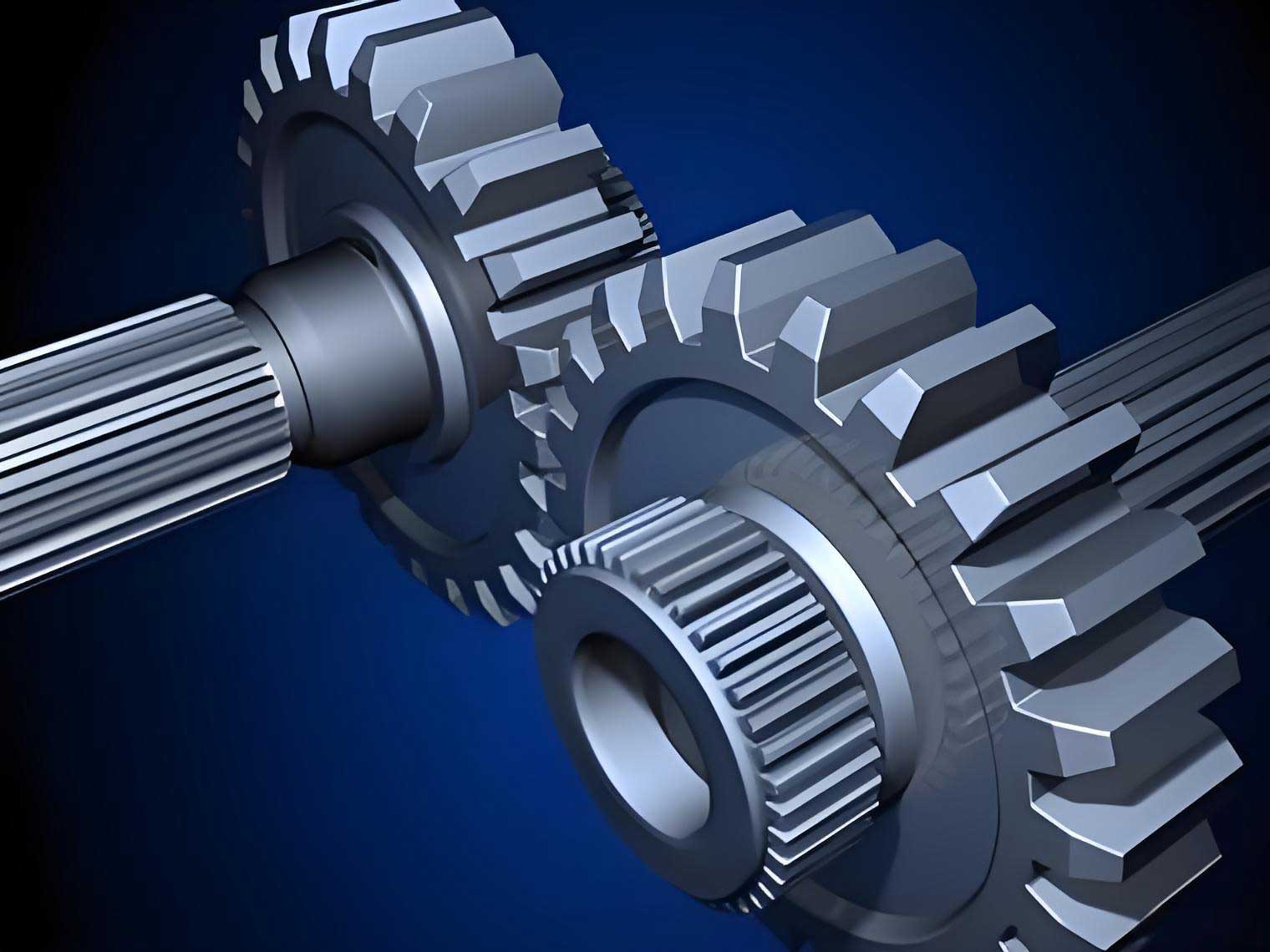
In the field of mechanical power transmission, the spur gear remains one of the most widely used components due to its high transmission efficiency, compact structure, and reliable operation. Throughout the long history of gear development, researchers have continuously sought methods to improve the load-carrying capacity of spur gear drives. Among the many approaches, optimizing tooth root stress distribution has proven to be one of the most effective strategies, as tooth root bending fatigue is the primary cause of tooth breakage in spur gear systems.
Conventional spur gear pairs are designed with equal module values for the driving and driven gears. However, according to the fundamental principles of gear meshing, the equality of modules is not a necessary condition for correct engagement. What truly matters is that the normal pitches of the two gears must be equal. This realization has led to the concept of the multi-modulus spur gear pair, in which the driving gear and driven gear possess different module values while still satisfying the meshing conditions. Such gear pairs offer additional design flexibility for optimizing tooth profile parameters and potentially improving load-carrying capacity.
Despite the potential advantages of multi-modulus spur gear pairs, the tooth root stress characteristics of these gear pairs have not been thoroughly investigated. In this study, I systematically analyzed the tooth root stress characteristics of multi-modulus involute spur gear pairs using both the plane cross section method and the broken-line section method. I also established three-dimensional solid models with accurate transition curve tooth profiles and conducted finite element simulations to validate the theoretical calculations. The influence of the module ratio and modification coefficients on the tooth root stress characteristics of the driving and driven gears was investigated in detail.
Parameter Calculation of Multi-Modulus Spur Gear Pairs
For a multi-modulus spur gear pair, the fundamental meshing condition requires that the normal pitches of the two gears be equal. This condition can be expressed as:
$$m_p \cos \alpha_p = m_g \cos \alpha_g$$
where \(m_p\) and \(m_g\) are the modules of the driving and driven gears respectively, and \(\alpha_p\) and \(\alpha_g\) are the pressure angles at the pitch circles of the driving and driven gears. I defined the module ratio as:
$$\delta_m = \frac{m_p}{m_g}$$
When the module ratio changes, the pressure angles must adjust accordingly to maintain the meshing condition. For instance, when \(\delta_m = 1.02\), the driving gear module \(m_p = 1.275\) mm and the pressure angle becomes \(\alpha_p = 22.89^\circ\), while the driven gear retains \(m_g = 1.25\) mm and \(\alpha_g = 20^\circ\).
Meshing Angle and Center Distance
For the multi-modulus spur gear pair, the operating meshing angle \(\alpha_v\) differs from both the driving and driven gear pressure angles. Based on the no-backlash meshing condition, I derived the meshing angle formula:
$$\text{inv}\,\alpha_v = \frac{2(x_p + x_g)}{z_p + z_g} + \frac{z_p\,\text{inv}\,\alpha_p + z_g\,\text{inv}\,\alpha_g}{z_p + z_g}$$
where \(x_p\) and \(x_g\) are the modification coefficients of the driving and driven gears, and \(z_p\) and \(z_g\) are the tooth numbers. The actual center distance is then calculated as:
$$a_1 = \frac{m_p z_p \cos \alpha_p + m_g z_g \cos \alpha_g}{2\cos \alpha_v}$$
Tooth Profile Parameters
The clearance coefficient and addendum coefficient of the multi-modulus spur gear pair must be modified to ensure proper meshing without interference. For the driven gear, I maintained standard values with \(c_2^* = 0.25\) and \(h_{a2}^* = 1.0\). For the driving gear, the clearance coefficient and addendum coefficient were determined as:
$$c_1^* = \frac{c_2^*}{\delta_m}$$
$$h_{a1}^* = \frac{h_{a2}^*}{\delta_m}$$
The addendum reduction coefficients \(\Delta y_1\) and \(\Delta y_2\) for the driving and driven gears respectively are expressed as:
$$\Delta y_1 = \frac{(z_p + z_g)\cos \alpha_p}{2\cos \alpha_v} – \frac{z_p + z_g}{2\delta_m} + x_p + x_g$$
$$\Delta y_2 = \frac{\delta_m(z_p + z_g)\cos \alpha_g}{2\cos \alpha_v} – \frac{z_p + z_g}{2} + x_p + x_g$$
Limiting Conditions for Modification Coefficients
When analyzing the tooth root stress characteristics of multi-modulus spur gear pairs, the modification coefficients must satisfy several constraints including the contact ratio condition, tooth tip thickness condition, and non-interference condition. The contact ratio must be greater than 1.2:
$$\varepsilon = \frac{m_p z_p(\tan \alpha_{ap} – \tan \alpha_v) + m_g z_g(\tan \alpha_{ag} – \tan \alpha_v)}{2\pi m_g \cos \alpha_g} > 1.2$$
The tooth tip thickness must remain above 0.25 times the module:
$$S_{a1} = m_p \left[ \frac{\pi}{2} + 2x_p \tan \alpha_p + z_p(\text{inv}\,\alpha_p – \text{inv}\,\alpha_{ap}) \right] > 0.25 m_p$$
Based on these limiting conditions, I determined the allowable ranges for the modification coefficients under different module ratios. For example, when investigating the combined effect of module ratio and driving gear modification coefficient, the driving gear modification coefficient ranged from -0.3 to 0.3 while the module ratio ranged from 0.98 to 1.06. When investigating the combined effect of module ratio and driven gear modification coefficient, the driven gear modification coefficient ranged from -0.4 to 0.4 while the module ratio ranged from 0.98 to 1.08.
Tooth Root Stress Calculation Methods
Two fundamentally different approaches exist for calculating tooth root stress in gear teeth: the plane cross section method and the broken-line section method. Each method defines the critical section differently and yields distinct results for multi-modulus spur gear pairs.
Plane Cross Section Method
The plane cross section method, which is the basis of the ISO standard, treats the critical section of the gear tooth as a single plane perpendicular to the tooth symmetry axis. The critical section is determined by the 30° tangent line method. For the multi-modulus spur gear pair, I derived the tooth root stress calculation formulas as:
$$\sigma_F^p = \sigma_{FO}^p K_A^p K_V^p K_{H\beta}^p K_{F\alpha}^p$$
$$\sigma_F^g = \sigma_{FO}^g K_A^g K_V^g K_{H\beta}^g K_{F\alpha}^g$$
where the basic stress values are:
$$\sigma_{FO}^p = \frac{F_t}{b_1 m_p} Y_F^p Y_S^p Y_\beta^p$$
$$\sigma_{FO}^g = \frac{F_t}{b_2 m_g} Y_F^g Y_S^g Y_\beta^g$$
The tooth form factor \(Y_F\) and stress correction factor \(Y_S\) are given by:
$$Y_F = \frac{6(h_F/m)\cos \alpha_F}{(\cos \alpha)(S_F/m)^2}$$
$$Y_S = (1.2 + 0.13L_k)\left(\frac{S_F}{2\rho_e}\right)^{\frac{1}{1.21 + 2.3/L_k}}$$
where \(h_F\) is the bending moment arm, \(S_F\) is the tooth thickness at the critical section, \(\alpha_F\) is the load angle, and \(\rho_e\) is the radius of curvature at the 30° tangent point.
Broken-Line Section Method
In reality, gear tooth cracks typically propagate along paths perpendicular to the tooth root transition curve, which means the critical section is not a single plane but rather a broken-line section. The broken-line section method determines the critical section as the line connecting two symmetric points on the transition curve, where the normal to the transition curve at each point intersects the tooth symmetry axis.
For the broken-line section method, the tooth root stress at any point on the transition curve of the multi-modulus spur gear pair can be calculated as:
$$\sigma_1 = \frac{T_1}{b_1 z_p Y_1} Y_{\sigma 1}$$
$$\sigma_2 = \frac{T_2}{b_2 z_g Y_2} Y_{\sigma 2}$$
where \(T_1\) and \(T_2\) are the input torques, \(Y_1\) and \(Y_2\) are half tooth thicknesses at the transition curve points, and \(Y_{\sigma 1}\) and \(Y_{\sigma 2}\) are the local stress coefficients:
$$Y_{\sigma 1} = \frac{\delta_m Y_1 \cos^2 \alpha_p}{\overline{GD_1} \cdot H_1 – Y_1 \cos \alpha_p (\delta_1 \cos \delta_1 \sin \delta_1 \cos \psi_1)}$$
$$Y_{\sigma 2} = \frac{Y_2 \cos^2 \alpha_g}{\overline{GD_2} \cdot H_2 – Y_2 \cos \alpha_g (\delta_2 \cos \delta_2 \sin \delta_2 \cos \psi_2)}$$
where \(\psi\) is the tangent angle at the point on the transition curve, and \(\overline{GD}\) is the distance between the intersection point of the force line with the gear symmetry axis and the intersection point of the normal to the transition curve with the gear symmetry axis.
Tooth Root Transition Curve Equation
To apply the broken-line section method to multi-modulus spur gear pairs, I derived the transition curve equations based on the generating method of gear manufacturing. When a rack-type cutter with a circular tip is used to generate the gear tooth profile, the transition curve on the gear tooth is generated by the circular arc portion of the cutter tip. For the driving gear of the multi-modulus spur gear pair, the transition curve equation is:
$$x_p = \frac{\delta_m z_p m_g}{2}(\phi_p \cos \phi_p – \sin \phi_p) + x_{11}^p \cos \phi_p + y_{11}^p \sin \phi_p$$
$$y_p = \frac{\delta_m z_p m_g}{2}(\phi_p \sin \phi_p – \cos \phi_p) – x_{11}^p \sin \phi_p + y_{11}^p \cos \phi_p$$
where the cutter tip coordinates are:
$$x_{11}^p = x_c^p + \rho_{f1}^* \delta_m m_g \cos \gamma_1$$
$$y_{11}^p = y_c^p – \rho_{f1}^* \delta_m m_g \sin \gamma_1$$
For the driven gear, the transition curve equation is:
$$x_g = \frac{z_g m_g}{2}(\phi_g \cos \phi_g – \sin \phi_g) + x_{11}^g \cos \phi_g + y_{11}^g \sin \phi_g$$
$$y_g = \frac{z_g m_g}{2}(\phi_g \sin \phi_g – \cos \phi_g) – x_{11}^g \sin \phi_g + y_{11}^g \cos \phi_g$$
The rolling angle \(\phi\) ranges from the initial value at the root circle to the final value at the start of the involute profile. This transition curve equation enabled me to establish accurate gear tooth profiles for both theoretical calculations and finite element modeling.
Tooth Root Stress Characteristic Analysis
To investigate the tooth root stress characteristics of multi-modulus spur gear pairs, I defined a set of baseline parameters. The driven gear module was maintained at \(m_g = 1.25\) mm with a pressure angle \(\alpha_g = 20^\circ\), clearance coefficient \(c_2^* = 0.25\), and addendum coefficient \(h_{a2}^* = 1.0\). The tooth numbers of the driving and driven gears were 19 and 23 respectively. The input power was 1.64 kW at a speed of 1750 rpm, and the face width of both gears was 16 mm. The input torque was 8949 N·mm for the finite element simulations.
Table 1 shows the example parameters for the multi-modulus spur gear pair calculations.
| No. | \(m_p\) (mm) | \(\alpha_p\) (°) | \(m_g\) (mm) | \(\alpha_g\) (°) | \(\delta_m\) |
|---|---|---|---|---|---|
| 1 | 1.2250 | 16.49 | 1.25 | 20 | 0.98 |
| 2 | 1.2375 | 18.34 | 0.99 | ||
| 3 | 1.2500 | 20.00 | 1.00 | ||
| 4 | 1.2625 | 21.50 | 1.01 | ||
| 5 | 1.2750 | 22.89 | 1.02 | ||
| 6 | 1.2875 | 24.17 | 1.03 | ||
| 7 | 1.3000 | 25.37 | 1.04 | ||
| 8 | 1.3125 | 26.50 | 1.05 | ||
| 9 | 1.3250 | 27.56 | 1.06 | ||
| 10 | 1.3375 | 28.57 | 1.07 | ||
| 11 | 1.3500 | 29.53 | 1.08 |
Stress Characteristics Based on Plane Cross Section Method
Using the plane cross section method, I first analyzed the effect of module ratio alone on the tooth root peak stress. My calculations showed that as the module ratio increased from 0.98 to 1.08, the driving gear root peak stress decreased continuously, while the driven gear root peak stress increased. This is because increasing the module ratio enlarges the driving gear tooth dimensions, increasing the section modulus and reducing stress concentration, while the driven gear experiences an increase in the load angle and bending moment arm.
When the module ratio and driving gear modification coefficient were varied simultaneously, I obtained the driving gear root peak stress values as shown in Table 2.
| \(\delta_m\) | \(x_p\) | ||||||
|---|---|---|---|---|---|---|---|
| -0.3 | -0.2 | -0.1 | 0 | 0.1 | 0.2 | 0.3 | |
| 0.98 | 219.2 | 206.6 | 196.9 | 189.4 | 183.8 | 179.7 | 176.8 |
| 1.00 | 180.7 | 173.5 | 168.0 | 164.0 | 161.1 | 159.1 | 157.8 |
| 1.02 | 156.6 | 152.5 | 149.4 | 147.1 | 145.7 | 144.8 | 144.4 |
| 1.04 | 140.6 | 138.1 | 136.3 | 135.2 | 134.5 | 134.4 | 134.3 |
| 1.06 | 129.3 | 127.8 | 126.8 | 126.2 | 126.0 | 126.1 | 126.4 |
From Table 2, I observed that when the module ratio ranged from 0.98 to 1.04, the driving gear root peak stress decreased monotonically with increasing modification coefficient. However, at module ratios of 1.05 and 1.06, the peak stress initially decreased and then increased as the modification coefficient increased. This non-monotonic behavior indicates that the 30° tangent section does not always correspond to the true critical section with maximum stress, which motivated my use of the broken-line section method.
The driven gear root peak stress under the same parameter combinations is shown in Table 3.
| \(\delta_m\) | \(x_p\) | ||||||
|---|---|---|---|---|---|---|---|
| -0.3 | -0.2 | -0.1 | 0 | 0.1 | 0.2 | 0.3 | |
| 0.98 | 116.6 | 120.1 | 123.2 | 126.0 | 128.7 | 131.2 | 133.5 |
| 1.00 | 121.5 | 125.1 | 128.5 | 131.5 | 134.4 | 137.1 | 139.6 |
| 1.02 | 127.0 | 130.7 | 134.0 | 137.2 | 140.1 | 142.9 | 145.5 |
| 1.04 | 132.7 | 136.3 | 139.6 | 142.8 | 145.7 | 148.5 | 151.1 |
| 1.06 | 138.3 | 141.8 | 145.1 | 148.2 | 151.1 | 153.9 | 156.6 |
Stress Characteristics Based on Broken-Line Section Method
The broken-line section method allowed me to obtain the complete stress distribution along the tooth root transition curve. I found that the tooth root stress on both the driving and driven gears first increased and then decreased as the tangent angle increased. This distribution pattern was consistent across all module ratios.
The tooth root stress distribution on the driving gear was markedly affected by the module ratio. As the module ratio increased, the stress distribution curve shifted downward, indicating a general reduction in tooth root stress. When the module ratio increased from 0.98 to 1.08, the peak stress location varied, but consistently remained within the vicinity of the 30° tangent angle position. The shifted position of the peak stress explains why the plane cross section method sometimes yielded different conclusions regarding stress variation trends.
Table 4 presents the driving gear root peak stress values obtained from the broken-line section method.
| \(\delta_m\) | \(x_p\) | ||||||
|---|---|---|---|---|---|---|---|
| -0.3 | -0.2 | -0.1 | 0 | 0.1 | 0.2 | 0.3 | |
| 0.98 | 151.0 | 140.1 | 131.8 | 125.7 | 121.1 | 117.8 | 115.7 |
| 1.00 | 121.9 | 115.7 | 111.0 | 107.5 | 105.0 | 103.3 | 102.2 |
| 1.02 | 105.0 | 101.1 | 98.24 | 96.09 | 94.60 | 93.66 | 93.20 |
| 1.04 | 94.13 | 91.59 | 89.67 | 88.28 | 87.36 | 86.84 | 86.66 |
| 1.06 | 86.78 | 84.98 | 83.62 | 82.67 | 82.05 | 81.75 | 81.71 |
Unlike the plane cross section method, the broken-line section method revealed a monotonic decrease in the driving gear root peak stress with increasing modification coefficient across all module ratios studied. The maximum reduction occurred at \(\delta_m = 0.98\), where the peak stress decreased by 35.3 MPa when the modification coefficient changed from -0.3 to 0.3.
Table 5 shows the corresponding driven gear root peak stress values.
| \(\delta_m\) | \(x_p\) | ||||||
|---|---|---|---|---|---|---|---|
| -0.3 | -0.2 | -0.1 | 0 | 0.1 | 0.2 | 0.3 | |
| 0.98 | 92.42 | 94.90 | 97.24 | 99.47 | 101.60 | 103.70 | 105.70 |
| 1.00 | 96.08 | 98.83 | 101.40 | 103.90 | 106.30 | 108.60 | 110.80 |
| 1.02 | 100.40 | 103.30 | 106.00 | 108.60 | 111.10 | 113.60 | 116.00 |
| 1.04 | 105.00 | 107.90 | 110.80 | 113.50 | 116.10 | 118.70 | 121.10 |
| 1.06 | 109.80 | 112.80 | 115.60 | 118.40 | 121.10 | 123.70 | 126.30 |
Combined Effect of Module Ratio and Driven Gear Modification Coefficient
I also investigated the combined effect of the module ratio and the driven gear modification coefficient on the tooth root stress characteristics of the multi-modulus spur gear pair. The driving gear modification coefficient was maintained at zero for this analysis. Table 6 presents the driving gear root peak stress values.
| \(\delta_m\) | \(x_g\) | ||||||||
|---|---|---|---|---|---|---|---|---|---|
| -0.4 | -0.3 | -0.2 | -0.1 | 0 | 0.1 | 0.2 | 0.3 | 0.4 | |
| 0.98 | 112.16 | 116.01 | 119.47 | 122.67 | 125.66 | 128.49 | 131.21 | 133.82 | 136.35 |
| 1.00 | 97.39 | 100.19 | 102.78 | 105.21 | 107.53 | 109.74 | 111.88 | 113.97 | 116.00 |
| 1.02 | 88.42 | 90.47 | 92.42 | 94.28 | 96.09 | 97.85 | 99.58 | 101.26 | 102.94 |
| 1.04 | 82.39 | 83.91 | 85.40 | 86.85 | 88.28 | 89.70 | 91.10 | 92.50 | 93.89 |
| 1.06 | 78.06 | 79.22 | 80.36 | 81.51 | 82.67 | 83.82 | 84.99 | 86.16 | 87.34 |
| 1.08 | 74.84 | 75.72 | 76.62 | 77.55 | 78.49 | 79.44 | 80.42 | 81.42 | 82.44 |
The results show that with the module ratio held constant, the driving gear root peak stress increased monotonically as the driven gear modification coefficient increased. When the driven gear modification coefficient remained constant, the driving gear root peak stress decreased as the module ratio increased. The module ratio had a more pronounced effect on the driving gear root peak stress compared to the driven gear modification coefficient.
Tangent Angle at Peak Stress Position
An important finding of my analysis is that the tangent angle corresponding to the tooth root peak stress is not consistently at 30°. Tables 7 and 8 show the tangent angle positions for the driving and driven gears under different parameter combinations.
| \(\delta_m\) | \(x_p\) | ||||||
|---|---|---|---|---|---|---|---|
| -0.3 | -0.2 | -0.1 | 0 | 0.1 | 0.2 | 0.3 | |
| 0.98 | 22.61 | 23.96 | 25.72 | 26.57 | 27.46 | 28.01 | 28.30 |
| 1.00 | 24.75 | 25.77 | 27.32 | 28.18 | 28.90 | 28.99 | 29.41 |
| 1.02 | 27.38 | 28.19 | 28.85 | 29.33 | 29.58 | 29.72 | 29.73 |
| 1.04 | 28.49 | 29.06 | 29.63 | 30.00 | 30.08 | 30.01 | 29.72 |
| 1.06 | 29.31 | 29.79 | 30.05 | 30.23 | 30.31 | 30.24 | 29.90 |
| \(\delta_m\) | \(x_p\) | ||||||
|---|---|---|---|---|---|---|---|
| -0.3 | -0.2 | -0.1 | 0 | 0.1 | 0.2 | 0.3 | |
| 0.98 | 31.52 | 30.90 | 30.69 | 30.09 | 29.89 | 29.10 | 28.71 |
| 1.00 | 30.69 | 30.09 | 29.69 | 28.90 | 28.52 | 28.14 | 27.57 |
| 1.02 | 29.69 | 29.29 | 28.57 | 28.32 | 27.57 | 27.20 | 27.02 |
| 1.04 | 28.71 | 28.32 | 27.76 | 27.20 | 26.83 | 26.47 | 25.93 |
| 1.06 | 27.95 | 27.38 | 26.83 | 26.29 | 25.93 | 25.58 | 25.23 |
These tables clearly show that the peak stress position varies substantially with both the module ratio and the modification coefficient. For the driving gear, the tangent angle at peak stress generally increases as the module ratio increases, while for the driven gear, it decreases. When the module ratio ranges from 0.98 to 1.03, the driving gear peak stress tangent angle remains below 30°, and the plane cross section method predictions align with the broken-line section method results. However, at higher module ratios (1.04 to 1.06), the tangent angle can exceed 30°, which explains the divergent predictions between the two methods.
Finite Element Modeling and Simulation
To validate the theoretical calculations, I established accurate three-dimensional solid models of the multi-modulus spur gear pairs. The key challenge was creating accurate transition curve tooth profiles that change with the tooth profile parameters. I solved this problem by using MATLAB to generate the transition curve coordinates based on the derived equations, then importing these coordinates into SolidWorks to construct the gear tooth profiles.
The modeling procedure involved several key steps. First, I calculated the gear profile parameters using equations (2-1) through (2-15). Second, I developed a MATLAB program to compute the transition curve data points based on equations (3-22) through (3-25). Third, I imported the point cloud data into SolidWorks and fitted the transition curves through the data points. Fourth, I constructed the complete tooth profile by combining the addendum circle, involute curve, transition curve, and dedendum circle. Finally, I assembled the driving and driven gears at the calculated actual center distance and verified that no interference existed.
For the finite element analysis, I used static structural analysis. The driving gear was constrained to rotate only about the y-axis, while the driven gear was fully fixed. Contact between the gears was defined as frictional contact with a friction coefficient of 0.2. The mesh size was set to 0.5 mm for the overall model and refined to 0.1 mm at the transition curve surfaces where the tooth root stress was to be measured. The input torque was 8949 N·mm applied clockwise on the driving gear.
I conducted simulations for different module ratios and driving gear modification coefficients, with the load applied at the single-tooth engagement upper bound point. Table 9 presents the finite element simulation results for the driving gear root peak stress.
| \(\delta_m\) | \(x_p\) | ||||||
|---|---|---|---|---|---|---|---|
| -0.3 | -0.2 | -0.1 | 0 | 0.1 | 0.2 | 0.3 | |
| 0.98 | 148.07 | 140.41 | 132.36 | 124.94 | 120.06 | 116.33 | 115.49 |
| 0.99 | 142.81 | 127.93 | 122.49 | 118.17 | 115.23 | 113.91 | 110.07 |
| 1.00 | 123.23 | 117.43 | 111.55 | 110.27 | 109.62 | 105.61 | 101.40 |
| 1.01 | 112.15 | 111.27 | 106.50 | 106.37 | 103.67 | 101.86 | 99.61 |
| 1.02 | 107.25 | 102.15 | 100.84 | 100.07 | 95.31 | 94.17 | 94.07 |
| 1.03 | 100.29 | 97.72 | 96.32 | 95.99 | 94.99 | 93.94 | 89.91 |
| 1.04 | 96.28 | 95.77 | 95.32 | 95.05 | 94.01 | 92.65 | 89.70 |
| 1.05 | 96.24 | 94.25 | 93.77 | 91.32 | 90.95 | 88.91 | 86.36 |
| 1.06 | 94.69 | 93.15 | 90.21 | 89.92 | 88.46 | 86.75 | 84.03 |
From Table 9, I observed that the finite element simulation results confirm the monotonic decreasing trend of the driving gear root peak stress with increasing modification coefficient. This finding aligns perfectly with the broken-line section method prediction and contradicts the non-monotonic trend suggested by the plane cross section method at higher module ratios.
Table 10 presents the corresponding finite element simulation results for the driven gear root peak stress.
| \(\delta_m\) | \(x_p\) | ||||||
|---|---|---|---|---|---|---|---|
| -0.3 | -0.2 | -0.1 | 0 | 0.1 | 0.2 | 0.3 | |
| 0.98 | 89.66 | 91.63 | 99.82 | 100.27 | 102.20 | 118.40 | 118.70 |
| 0.99 | 92.43 | 97.77 | 101.32 | 102.82 | 105.08 | 120.60 | 120.93 |
| 1.00 | 98.68 | 99.90 | 102.42 | 105.43 | 121.17 | 122.29 | 123.28 |
| 1.01 | 101.27 | 103.58 | 116.47 | 119.55 | 121.38 | 122.31 | 128.22 |
| 1.02 | 113.26 | 113.98 | 118.52 | 120.91 | 121.59 | 122.97 | 134.44 |
| 1.03 | 113.48 | 116.39 | 119.11 | 121.60 | 121.98 | 123.05 | 134.61 |
| 1.04 | 113.72 | 117.09 | 120.20 | 121.84 | 122.66 | 128.79 | 136.08 |
| 1.05 | 115.65 | 119.85 | 121.42 | 122.68 | 133.50 | 134.54 | 136.27 |
| 1.06 | 118.01 | 120.62 | 122.28 | 130.68 | 133.98 | 135.90 | 137.75 |
Comparison Between Simulation and Theoretical Calculation
I compared the finite element simulation results with the theoretical calculations to evaluate the accuracy of both methods. The comparison revealed that the broken-line section method provides significantly better agreement with the finite element simulation than the plane cross section method.
Table 11 shows the difference between the finite element simulation data and the broken-line section method calculations for the driving gear root peak stress.
| \(\delta_m\) | \(x_p\) | ||||||
|---|---|---|---|---|---|---|---|
| -0.3 | -0.2 | -0.1 | 0 | 0.1 | 0.2 | 0.3 | |
| 0.98 | 2.93 | -0.31 | -0.56 | 0.76 | 1.04 | 1.47 | 0.21 |
| 0.99 | -8.41 | -1.73 | -2.39 | -2.77 | -3.13 | -4.21 | -1.87 |
| 1.00 | -1.33 | -1.73 | -0.55 | -2.77 | -4.62 | -2.31 | 0.80 |
| 1.01 | 0.25 | -3.67 | -2.60 | -5.17 | -4.39 | -3.85 | -2.30 |
| 1.02 | -2.25 | -1.05 | -2.60 | -3.98 | -0.71 | -0.51 | -0.87 |
| 1.03 | -1.31 | -1.82 | -2.77 | -4.15 | -4.32 | -3.97 | -0.22 |
| 1.04 | -2.15 | -4.18 | -5.65 | -6.77 | -6.65 | -5.81 | -3.04 |
| 1.05 | -6.13 | -6.26 | -7.37 | -6.07 | -6.44 | -4.79 | -2.34 |
| 1.06 | -7.91 | -8.17 | -6.59 | -7.25 | -6.41 | -5.00 | -2.32 |
The differences range from -8.41 MPa to +2.93 MPa, corresponding to relative errors between 0.18% and 8.77%. In contrast, the differences between the finite element simulation and the plane cross section method for the same gear and conditions ranged from 34.6 MPa to 71.1 MPa, corresponding to errors between 36.6% and 55.6%. This substantial discrepancy confirms that the plane cross section method, which assumes a fixed 30° critical section, does not accurately capture the tooth root peak stress in multi-modulus spur gear pairs.
Table 12 presents the difference between the finite element simulation data and the broken-line section method calculations for the driven gear root peak stress.
| \(\delta_m\) | \(x_p\) | ||||||
|---|---|---|---|---|---|---|---|
| -0.3 | -0.2 | -0.1 | 0 | 0.1 | 0.2 | 0.3 | |
| 0.98 | 2.76 | 3.27 | -2.58 | -0.80 | -0.60 | -14.70 | -13.00 |
| 0.99 | 1.71 | -0.99 | -2.05 | -1.22 | -1.18 | -14.50 | -12.63 |
| 1.00 | -2.60 | -1.07 | -1.02 | -1.53 | -14.87 | -13.69 | -12.48 |
| 1.01 | -3.10 | -2.58 | -12.77 | -13.35 | -12.68 | -11.21 | -14.82 |
| 1.02 | -12.86 | -10.68 | -12.52 | -12.31 | -10.49 | -9.37 | -18.44 |
| 1.03 | -10.88 | -10.79 | -10.71 | -10.60 | -8.38 | -6.95 | -16.01 |
| 1.04 | -8.72 | -9.19 | -9.40 | -8.34 | -6.56 | -10.09 | -14.98 |
| 1.05 | -8.25 | -9.55 | -8.22 | -6.78 | -14.90 | -13.34 | -12.57 |
| 1.06 | -8.21 | -7.82 | -6.68 | -12.28 | -12.88 | -12.20 | -11.45 |
For the driven gear, the differences between the broken-line section method and the finite element simulation ranged from -18.44 MPa to +3.27 MPa, corresponding to errors between 0.59% and 13.72%. The plane cross section method generally overestimated the driven gear root peak stress, with differences between 11.06 MPa and 28.47 MPa.
The finite element simulation also confirmed the stress distribution pattern along the tooth root transition curve. The equivalent stress distribution obtained from the simulation showed that the tooth root stress first increased and then decreased as the tangent angle increased, which agrees with the broken-line section method prediction. The maximum stress occurred near the 30° tangent angle position but not exactly at it, further validating the necessity of using the broken-line section method for accurate multi-modulus spur gear pair analysis.
Conclusion
In this study, I systematically investigated the tooth root stress characteristics of multi-modulus involute spur gear pairs through theoretical calculations and finite element simulations. The key findings and conclusions are summarized as follows:
First, I derived the meshing parameter calculation formulas for multi-modulus spur gear pairs, including the meshing angle, actual center distance, clearance coefficient, and addendum coefficient. These formulas account for the module ratio and modification coefficients, providing a solid theoretical foundation for the design and analysis of multi-modulus spur gear pairs.
Second, I derived tooth root stress calculation formulas based on both the plane cross section method and the broken-line section method, specifically adapted for multi-modulus spur gear pairs. Additionally, I derived the tooth root transition curve equations for both the driving and driven gears based on the generating method of gear manufacturing.
Third, the tooth root stress characteristic analysis revealed that when the module ratio increases from 0.98 to 1.08, the driving gear root peak stress decreases while the driven gear root peak stress increases. Increasing the driving gear modification coefficient reduces the driving gear root peak stress but increases the driven gear root peak stress. The module ratio has a more pronounced effect on the tooth root stress than the modification coefficient.
Fourth, both the plane cross section and broken-line section methods showed that increasing the driven gear modification coefficient increases the driving gear root peak stress and decreases the driven gear root peak stress. The module ratio remains the dominant factor affecting the tooth root stress characteristics.
Fifth, the finite element simulations confirmed the tooth root stress distribution pattern along the transition curve and validated that the broken-line section method provides more accurate results than the plane cross section method for multi-modulus spur gear pairs. The differences between the broken-line section method calculations and finite element simulation results were within acceptable engineering accuracy, while the plane cross section method showed significant deviations.
Finally, the research demonstrates that the multi-modulus spur gear pair concept offers an additional degree of freedom for optimizing gear tooth root stress. By appropriately selecting the module ratio and modification coefficients, the tooth root stress of multi-modulus spur gear pairs can be effectively reduced, contributing to improved load-carrying capacity and longer service life of spur gear transmissions.