
Straight bevel gears are essential machine elements for transmitting motion and power between intersecting axes. Compared with helical and curved tooth bevel gears, straight bevel gears are much simpler in design and manufacture, and thus they are widely applied in various industrial fields including power generation, building materials, marine equipment, mining machinery, and national defense installations. In recent years, the demand for outsize straight bevel gears, whose outer diameter exceeds 3000 mm, has increased significantly. However, the machining technology and equipment for such large gears are mainly dependent on imports, which severely restricts the development of relevant domestic industries. The existing machining methods used for outsize straight bevel gears often suffer from low accuracy, low efficiency, and high cost. Therefore, it is of great importance to investigate a novel and economical machining approach for outsize straight bevel gears.
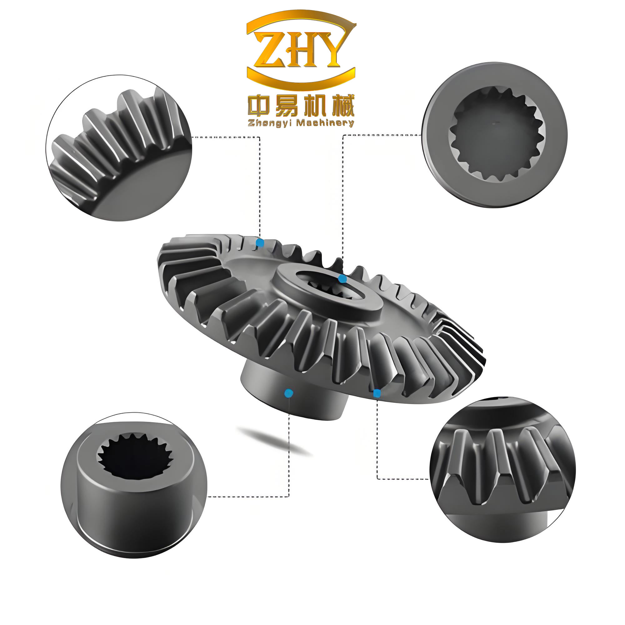
In this paper, I propose an envelope shaping method for outsize straight bevel gears based on the geometric characteristics of the theoretical tooth surface. The method uses a cutter with a straight cutting edge to generate a series of planes that envelope the theoretical tooth surface. The workpiece rotates continuously during the machining process, which significantly improves the machining efficiency and reduces the requirements on the driving motor. The proposed method abandons the traditional idea of a generating gear and makes the machining process more intuitive. In addition, the traditional method of calculating parameters using the equivalent spur gear at the large end is replaced by a direct calculation from the spherical involute, thereby avoiding theoretical calculation errors. The research lays a theoretical foundation for the design of numerical control planers for outsize straight bevel gears and promotes the progress of large gear machining technology.
1. Theoretical Tooth Surface of Straight Bevel Gear
1.1 Generation Principle
The theoretical tooth surface of a straight bevel gear is formed by a plane circle, called the generating plane, which rolls purely over the base cone. As shown in the classical theory, let the vertex of the base cone be point \(O\), and let the generating plane \(C\) be tangent to the base cone along the line \(AA’\). When the generating plane rolls over the base cone without slipping, the line \(AA’\) sweeps a curved surface known as the involute cone surface. The intersection of this surface with a sphere centered at \(O\) is a spherical involute. The actual tooth surface of a straight bevel gear can be regarded as a family of spherical involutes lying on different concentric spheres centered at the cone vertex. The spherical involute has the property that it cannot be developed into a plane curve, and therefore the tooth surface is a non-developable ruled surface.
1.2 Mathematical Model of the Tooth Surface
From the generation principle, the tooth surface of a straight bevel gear is a ruled surface. The large-end and small-end tooth profiles are two spherical involutes, which can be treated as the two directrices of the ruled surface. The straight generatrices are the cone elements connecting corresponding points on the two directrices. Consequently, the tooth surface can be expressed by the following parametric equation in ruled-surface form:
$$
\mathbf{S}(r,\varphi) = (1-r)\mathbf{W}(\varphi) + r\mathbf{Q}(\varphi), \quad 0\le r \le 1,
\tag{1}
$$
where \(r\) is the linear parameter along the generatrix, \(\varphi\) is the angular parameter of the spherical involute, \(\mathbf{Q}(\varphi)\) is the large-end tooth profile, and \(\mathbf{W}(\varphi)\) is the small-end tooth profile.
To establish the expressions for \(\mathbf{Q}(\varphi)\) and \(\mathbf{W}(\varphi)\), I constructed a fixed coordinate system \(S(x,y,z)\) with origin at the cone vertex \(O\), the \(z\)-axis coinciding with the base cone axis, and the \(x\)-axis parallel to the radius of the base cone at the starting point of the spherical involute. An auxiliary coordinate system \(S_1(x_1,y_1,z_1)\) is also adopted, where the \(z_1\)-axis is the instantaneous axis of rotation of the generating plane and the origin is the same as that of \(S\). The transformation between the two coordinate systems is:
$$
\begin{bmatrix}
x\\ y\\ z\\ 1
\end{bmatrix}
=
\begin{bmatrix}
\sin\phi & \cos\phi & 0 & 0\\
-\cos\phi & \sin\phi & 0 & 0\\
0 & 0 & 1 & 0\\
0 & 0 & 0 & 1
\end{bmatrix}
\begin{bmatrix}
1 & 0 & 0 & 0\\
0 & \cos\delta_b & -\sin\delta_b & 0\\
0 & \sin\delta_b & \cos\delta_b & 0\\
0 & 0 & 0 & 1
\end{bmatrix}
\begin{bmatrix}
x_1\\ y_1\\ z_1\\ 1
\end{bmatrix},
\tag{2}
$$
where \(\delta_b\) is the base cone angle. In the coordinate system \(S_1\), a point \(K\) on the generating plane is expressed as:
$$
\begin{cases}
x_1 = R\sin\psi,\\
y_1 = 0,\\
z_1 = R\cos\psi,
\end{cases}
\tag{3}
$$
where \(R\) is the cone distance and \(\psi\) is the angle between the line \(OK\) and the instantaneous axis \(ON\). Pure rolling of the generating plane over the base cone gives:
$$
R\psi = R\phi\sin\delta_b,
\tag{4}
$$
and hence
$$
\psi = \phi\sin\delta_b.
\tag{5}
$$
Substituting equation (5) into equation (3) and then applying the coordinate transformation (2), the large-end tooth profile can be expressed in the fixed coordinate system as:
$$
\mathbf{Q}(\varphi) =
\begin{cases}
Q_x(\varphi) = R[\cos(\varphi\sin\delta_b)\sin\delta_b\cos\phi + \sin(\varphi\sin\delta_b)\sin\phi],\\[4pt]
Q_y(\varphi) = R[\cos(\varphi\sin\delta_b)\sin\delta_b\sin\phi – \sin(\varphi\sin\delta_b)\cos\phi],\\[4pt]
Q_z(\varphi) = R\cos(\varphi\sin\delta_b)\cos\delta_b.
\end{cases}
\tag{6}
$$
Similarly, the small-end tooth profile is obtained by replacing \(R\) with \(R-B\), where \(B\) is the face width:
$$
\mathbf{W}(\varphi) =
\begin{cases}
W_x(\varphi) = (R-B)[\cos(\varphi\sin\delta_b)\sin\delta_b\cos\phi + \sin(\varphi\sin\delta_b)\sin\phi],\\[4pt]
W_y(\varphi) = (R-B)[\cos(\varphi\sin\delta_b)\sin\delta_b\sin\phi – \sin(\varphi\sin\delta_b)\cos\phi],\\[4pt]
W_z(\varphi) = (R-B)\cos(\varphi\sin\delta_b)\cos\delta_b.
\end{cases}
\tag{7}
$$
Equations (1), (6), and (7) completely define the theoretical tooth surface of a straight bevel gear. The angular parameter \(\varphi\) lies in the range
$$
0 \le \varphi \le \frac{\arccos\left(\frac{\cos\delta_a}{\cos\delta_b}\right)}{\sin\delta_b},
\tag{8}
$$
where \(\delta_a\) is the face cone angle.
1.3 Geometric Characteristics
To investigate the convexity of the theoretical tooth surface, I analyzed the partial derivatives of equation (1). The derivative with respect to \(r\) is:
$$
\mathbf{S}_r = \mathbf{Q}(\varphi)-\mathbf{W}(\varphi),
\tag{9}
$$
which is a constant vector for a fixed \(\varphi\). This means that all points on the same straight generatrix have the same tangent vector along the \(r\)-direction, and therefore the surface is indeed a ruled surface generated by straight lines.
The derivative with respect to \(\varphi\) is:
$$
\mathbf{S}_\varphi = (1-r)\mathbf{W}'(\varphi) + r\mathbf{Q}'(\varphi).
\tag{10}
$$
Substituting the relation \(\mathbf{W}'(\varphi) = \frac{R-B}{R}\mathbf{Q}'(\varphi)\) yields:
$$
\mathbf{S}_\varphi = \left[(1-r)\frac{R-B}{R} + r\right]\mathbf{Q}'(\varphi).
\tag{11}
$$
The vector \(\mathbf{S}_\varphi\) determines the tangent direction along the profile direction. By projecting \(\mathbf{S}_\varphi\) onto the \(xOy\) plane, the angle \(\eta\) between the projection and the \(x\)-axis satisfies:
$$
\cos\eta = \frac{Q’_x}{\sqrt{(Q’_x)^2 + (Q’_y)^2}}.
\tag{12}
$$
Taking the derivative of \(\cos\eta\) with respect to \(\varphi\), I obtained:
$$
\frac{d(\cos\eta)}{d\varphi} = \frac{Q’_y(Q’_yQ”_x – Q’_xQ”_y)}{[(Q’_x)^2+(Q’_y)^2]^{3/2}}
= \frac{R’\sin^2(\varphi\sin\delta_b)\sin\delta_b(\sin^2\delta_b-1)\cos(\varphi\sin\delta_b)}{[(Q’_x)^2+(Q’_y)^2]^{3/2}}.
\tag{13}
$$
Since the denominator is always positive and \(\sin^2\delta_b<1\), the derivative is always negative. Hence \(\cos\eta\) is a monotonically decreasing function, which indicates that the direction of \(\mathbf{S}_\varphi\) changes monotonically. This result reveals that the theoretical tooth surface of a straight bevel gear is a convex surface. All tangent planes that are tangent to the tooth surface along a straight generatrix lie on the same side of the surface. This convexity makes it feasible to approximate the theoretical tooth surface by a series of planes, i.e., a polyhedral surface.
2. Envelope Shaping Principle and Cutting Method
2.1 Principle of Envelope Shaping
Because the theoretical tooth surface is convex, it can be approximated by a polyhedral surface formed by multiple planes. Each plane is tangent to the theoretical tooth surface along one straight generatrix. Consecutive planes intersect along straight lines, and when the number of planes is sufficiently large, the polyhedral surface approaches the theoretical tooth surface to within an acceptable tolerance. In machining, each plane is generated by the straight cutting edge of a throwaway blade as it moves along a straight generatrix of the theoretical tooth surface. Thus, by successively cutting a series of tangent planes, the final machined tooth surface is a multi-faceted surface that envelopes the theoretical tooth surface.
2.2 Cutting Method
In the proposed method, the work gear is mounted with its pitch cone generatrix horizontal. The cutter moves in the horizontal direction (the main cutting direction) while the workpiece rotates continuously. The cutting edge of the blade is straight, and the blade is a rhombic indexable insert with a nose angle \(\gamma\). The cutting process proceeds from the large end to the small end of the gear, and from the tooth top to the tooth root. Before each cutting pass, the cutter is positioned so that its cutting edge is tangent to the projection of the large-end tooth profile onto a projection plane. This projection plane is parallel to the cutting edge plane and passes through the cone vertex. After the cutter is set, the workpiece begins to rotate, and the cutter moves along the straight generatrix corresponding to the current cut-in point. During this movement, the cutter swings and translates in the machine \(X\) and \(Y\) directions to maintain tangency with the rotating tooth surface. The swept surface of the cutting edge is therefore a plane tangent to the theoretical tooth surface along a generatrix. By repeating this process for different cut-in points, a polyhedral surface is obtained.
3. Machine Motions and Motion Models
3.1 Coordinate Systems and Projection Plane
I established a machine coordinate system as shown in the original design, where the \(Z\)-axis is the direction of the ram main motion, the \(X\)-axis is horizontal and perpendicular to \(Z\), and the \(Y\)-axis is vertical. The workpiece coordinate system \(S\) is attached to the gear during its theoretical generation. The projection plane is determined by its normal vector \(\mathbf{n}\), which is along the pitch cone generatrix. The normal vector can be expressed in the workpiece coordinate system as:
$$
\mathbf{n} = (R\sin\delta\cos\theta,\; R\sin\delta\sin\theta,\; R\cos\delta),
\tag{14}
$$
where \(\delta\) is the pitch angle and \(\theta\) is the angle between the projection of the workpiece axis on the \(xOy\) plane and the \(x\)-axis. The angle \(\theta\) is calculated from the base cone geometry and the circular tooth thickness at the pitch cone:
$$
\theta = \arccos\left[\frac{Q_x\left(\varphi_c\right)}{R\sin\delta}\right] + \frac{\pi m}{4R\sin\delta},
\tag{15}
$$
where \(\varphi_c\) corresponds to the spherical involute point on the pitch cone and \(m\) is the large-end module.
3.2 Cut-in Point Positions
The tooth flank is machined in several passes. The cut-in points are selected by dividing the angle between the face cone and root cone into \(k\) equal intervals, where \(k\) is the number of enveloping planes. The cone angle at the \(n\)-th cut-in point is:
$$
\delta_n = \delta_a – n\frac{\delta_a-\delta_f}{k-1}, \quad n=0,1,2,\ldots,k-1.
\tag{16}
$$
The corresponding parameter \(\varphi_n\) on the large-end tooth profile is obtained from
$$
\varphi_n = \frac{\arccos\left(\frac{\cos\delta_n}{\cos\delta_b}\right)}{\sin\delta_b}.
\tag{17}
$$
The coordinates of the cut-in point are then given by substituting \(\varphi_n\) into equation (6). To align the generatrix at the cut-in point with the workpiece axis projection in the projection plane, the workpiece must rotate by an angle \(\Delta\theta_n\). This angle is determined by the chordal tooth thickness at the cut-in point. Instead of using the equivalent spur gear approximation, I compute the chordal tooth thickness exactly from the spherical involute. Introducing an auxiliary coordinate system \(S_2\) whose \(z_2\)-axis coincides with the \(z\)-axis and whose \(x_2\)-axis forms an angle \(\theta\) with the \(x\)-axis, the \(y_2\)-coordinate of the large-end profile gives the chordal half-thickness. The exact chordal tooth thickness is:
$$
S_n = 2\left[Q_y(\varphi_n)\cos\theta – Q_x(\varphi_n)\sin\theta\right].
\tag{18}
$$
The workpiece rotation angle is then:
$$
\Delta\theta_n = \arcsin\left(\frac{S_n}{2R\sin\delta_n}\right).
\tag{19}
$$
After rotating the workpiece by \(\Delta\theta_n\), the large-end tooth profile in the workpiece coordinate system becomes:
$$
\mathbf{P}(\varphi) =
\begin{bmatrix}
\cos\Delta\theta_n & \sin\Delta\theta_n & 0\\
-\sin\Delta\theta_n & \cos\Delta\theta_n & 0\\
0 & 0 & 1
\end{bmatrix}
\mathbf{Q}(\varphi).
\tag{20}
$$
3.3 Projection of the Large-End Tooth Profile
To position the cutter correctly, I project the rotated large-end tooth profile onto the projection plane whose normal vector is given by equation (14). For any point \((P_x, P_y, P_z)\) on the profile, the projection onto the plane is obtained by drawing a line perpendicular to the plane. The projected coordinates are:
$$
\begin{cases}
x_t = P_x – s_0 R\sin\delta\cos\theta,\\
y_t = P_y – s_0 R\sin\delta\sin\theta,\\
z_t = P_z – s_0 R\cos\delta,
\end{cases}
\tag{21}
$$
where
$$
s_0 = \frac{P_x\sin\delta\cos\theta + P_y\sin\delta\sin\theta + P_z\cos\delta}{R}.
\tag{22}
$$
The tangent vector of the projected profile at the cut-in point is obtained by differentiating equation (21) with respect to \(\varphi\). The angle \(\lambda_n\) between this tangent vector and the workpiece axis projection (whose unit vector is \((\cos\delta\cos\theta,\cos\delta\sin\theta,\sin\delta)\)) is:
$$
\lambda_n = \arccos\left[\frac{x’_t\cos\delta\cos\theta + y’_t\cos\delta\sin\theta + z’_t\sin\delta}{\sqrt{(x’_t)^2+(y’_t)^2+(z’_t)^2}}\right].
\tag{23}
$$
The initial swing angle of the cutter is then:
$$
\beta_n =
\begin{cases}
\gamma – \lambda_n, & n=0,\\
\beta_{n-1} – \lambda_n, & n>0,
\end{cases}
\tag{24}
$$
where \(\gamma\) is the nose angle of the rhombic blade.
3.4 Tooth Surface Forming Motions
During each cutting pass, the cutter must follow the moving generatrix while the workpiece rotates continuously. I divided the generatrix into \(N\) points. The ram displacement in the \(Z\)-direction is denoted by \(L_{Z(N)}\). The relationship between the ram motion and the workpiece rotation is:
$$
L_{Z(N)} = L’_{Z(N)} + r_{n(N)}(1-\cos\omega_1 t)\sin\delta_n,
\tag{25}
$$
where \(L’_{Z(N)}\) is the displacement when the workpiece is fixed, \(r_{n(N)}\) is the radial distance at the current point, \(\omega_1\) is the workpiece angular velocity, and \(t\) is the time. Since \(t = L_{Z(N)}/v_Z\), where \(v_Z\) is the ram velocity, equation (25) can be solved implicitly for \(L_{Z(N)}\).
The cutter must also swing about its pivot to maintain tangency with the rotating tooth surface. The required swing angle at the \(N\)-th point is:
$$
\beta_{n(N)} = \beta_n – \lambda_{n(N)}’,
\tag{26}
$$
where \(\lambda_{n(N)}’\) is the angle between the projection tangent of the current spherical involute and the workpiece axis projection. This angle is computed similarly to equation (23) but using the rotated expression of the spherical involute at the corresponding cone distance.
The compensating motions in the machine \(X\) and \(Y\) directions depend on the swing angle and the blade geometry. If \(\beta_n \ge \eta_n\), where \(\eta_n\) is the angle between the cutting edge and the line connecting the pivot to the tangency point, then:
$$
L_{Y(N)} = L_{Z(N)}\tan(\delta-\delta_n) – r_{n(N)}[1-\cos(\omega_1 t)] – l’_n[\cos(\beta_n-\eta_n) – \cos(\beta_n+\eta_n)],
\tag{27}
$$
$$
L_{X(N)} = r_{n(N)}\sin(\omega_1 t) + l’_n[\sin(\beta_n+\eta_n) – \sin(\beta_n-\eta_n)].
\tag{28}
$$
If \(\beta_n < \eta_n\), the corresponding expressions are:
$$
L_{Y(N)} = L_{Z(N)}\tan(\delta-\delta_n) + r_{n(N)}[1-\cos(\omega_1 t)] – l’_n[\cos(\beta_n+\eta_n) – \cos(\eta_n-\beta_n)],
\tag{29}
$$
$$
L_{X(N)} = r_{n(N)}\sin(\omega_1 t) + l’_n[\sin(\eta_n-\beta_n) – \sin(\beta_n+\eta_n)].
\tag{30}
$$
These motion models ensure that the cutting edge sweeps a plane tangent to the theoretical tooth surface along the entire generatrix while the workpiece rotates.
3.5 Envelope Accuracy and Control
The polyhedral surface formed by the enveloping planes deviates from the theoretical tooth surface. The maximum deviation occurs on the intersection lines of adjacent planes. To evaluate the envelope accuracy, I constructed the plane generated by the cutting edge for each pass. The plane equation is determined by the cutting edge direction vector \(\mathbf{T}_n\) and the generatrix direction vector \(\mathbf{F}_n\). The plane normal is:
$$
\mathbf{n}_n = \mathbf{T}_n \times \mathbf{F}_n.
\tag{31}
$$
The plane equation is:
$$
n_{nx}(x-P_x) + n_{ny}(y-P_y) + n_{nz}(z-P_z) = 0.
\tag{32}
$$
The intersection line of two adjacent planes is obtained by solving the two plane equations simultaneously. I denote this intersection line by \(L_i\). To compute the distance from a point on \(L_i\) to the theoretical tooth surface, I used a grid method. The tooth surface was discretized into a grid, and for each point on the intersection line, the closest grid point was found as an initial estimate. Then the grid was refined locally until the step was smaller than a prescribed tolerance. The resulting minimum distance was taken as the distance from that point to the surface. By repeating this process for all points on all intersection lines, I obtained a set of distances \(d_j\). The envelope accuracy \(\mu\) is defined as the maximum value of these distances:
$$
\mu = \max_{j} \{d_j\}, \quad j=1,2,\ldots,M(k-1).
\tag{33}
$$
If \(\mu\) exceeds the required tolerance, the number of enveloping planes \(k\) is increased, and the entire procedure is repeated. In this way, the machining accuracy can be controlled by adjusting the enveloping times.
3.6 Machine Motion Layout
The required motions include: the main ram motion along the \(Z\)-axis, the workpiece continuous rotation, the cutter swinging about a pivot, the cutter translation along the \(X\)-axis, and the cutter translation along the \(Y\)-axis. To avoid the inertia caused by moving a heavy workpiece, the two compensating motions (\(X\) and \(Y\)) are assigned to the cutter side, while the workpiece only rotates. The machine table can be tilted to accommodate different pitch angles and gear sizes, thereby increasing the versatility of the machine. A schematic layout is shown in the original study, but here I only summarize the conceptual arrangement: the ram carries the swivel head with the blade, the \(X\) and \(Y\) slides are mounted on the ram, and the workpiece spindle is mounted on an adjustable table. This layout ensures high stiffness and accurate coordination of the five motions.
4. Development of Calculation Software
The calculation of all machining parameters and envelope accuracy is mathematically complex and time-consuming if performed manually. To facilitate the practical application of the proposed method, I developed a dedicated calculation software package using MATLAB for numerical computation and Visual Basic (VB) for the graphical user interface. MATLAB provides powerful numerical functions, while VB offers a simple and efficient way to design interactive interfaces. I wrote the core computational algorithms as MATLAB M-files and then compiled them into COM components using the MATLAB COM Builder. These components were subsequently invoked from a VB-based front end.
The software architecture is divided into several modules:
- Input module – accepts the workpiece geometric parameters, machine parameters, and tool parameters.
- Computation module – performs tooth surface modeling, cut-in point calculation, projection computation, motion parameter calculation, plane generation, intersection line calculation, and envelope accuracy evaluation.
- Database module – stores and manages the parameter files of existing workpieces and their corresponding machining parameters. Microsoft Access format is used for data persistence.
- Result display module – presents the calculated cutting passes, motion tables, and envelope accuracy in a tabular format.
The total calculation procedure is illustrated in the flowchart in the original paper. The envelope accuracy calculation module updates the number of passes iteratively until the accuracy requirement is satisfied. The COM component interface is straightforward; in VB, I instantiate the component and call its methods to pass input parameters and retrieve output arrays. This mixed programming approach greatly shortens the development cycle and makes the software easy to maintain and upgrade.
5. Calculation Example
To verify the correctness and feasibility of the proposed envelope shaping method, I performed a numerical example using a large straight bevel gear with the following geometric parameters:
| Parameter | Symbol | Value |
|---|---|---|
| Number of teeth | \(z\) | 200 |
| Large-end module | \(m\) | 40 mm |
| Pressure angle | \(\alpha\) | 20° |
| Pitch angle | \(\delta\) | 84°43′ |
| Face width | \(B\) | 400 mm |
| Addendum coefficient | \(h_a^*\) | 1 |
| Clearance coefficient | \(c^*\) | 0.2 |
| Addendum | \(h_a\) | 40 mm |
| Dedendum | \(h_f\) | 48 mm |
| Cone distance | \(R\) | 4017.07 mm |
| Face cone angle | \(\delta_a\) | 85°17’26” |
| Root cone angle | \(\delta_f\) | 84°02’07” |
| Tool nose angle | \(\gamma\) | 35° |
| Required envelope accuracy | \(\mu_{req}\) | 0.03 mm |
Initially, I selected \(k=3\) as the number of enveloping planes. According to equation (16), the cut-in points have cone angles of 85°17’26”, 84°39’47”, and 84°02’07”. Their corresponding parameters \(\varphi_n\) and initial cutter swing angles \(\beta_n\) are listed below:
| Cut-in point \(n\) | Cone angle \(\delta_n\) | Parameter \(\varphi_n\) | Initial swing angle \(\beta_n\) |
|---|---|---|---|
| 0 | 85°17’26” | 2°38’22” | 0° |
| 1 | 84°39’47” | 2°28’44” | 0° |
| 2 | 84°02’07” | 2°15’47” | 0° |
The workpiece angular velocity was set to \(\omega_1 = 0.02\) rad/s. The ram velocity was chosen so that the total cutting time corresponded to the ram stroke. The computed motion displacements in the \(X\), \(Y\), and \(Z\) directions at selected points along the generatrix are summarized in the following table:
| Point along generatrix | \(L_X\) (mm) | \(L_Y\) (mm) | \(L_Z\) (mm) | ||||||
|---|---|---|---|---|---|---|---|---|---|
| pass 1 | pass 2 | pass 3 | pass 1 | pass 2 | pass 3 | pass 1 | pass 2 | pass 3 | |
| 1 | 0 | 0 | 0 | 0 | 0 | 0 | 0 | 0 | 0 |
| 5 | 1.644 | 1.643 | 1.641 | -0.839 | 0.084 | 1.006 | 84.207 | 84.211 | 84.205 |
| 10 | 3.600 | 3.597 | 3.593 | -1.887 | 0.189 | 2.264 | 189.466 | 189.475 | 189.462 |
| 15 | 5.446 | 5.441 | 5.435 | -2.935 | 0.293 | 3.521 | 294.726 | 294.741 | 294.720 |
| 20 | 7.182 | 7.175 | 7.167 | -3.984 | 0.398 | 4.779 | 399.987 | 400.007 | 399.979 |
Using the motion model, I constructed the three enveloping planes. Their equations in the workpiece coordinate system are:
$$
\begin{aligned}
\text{Plane 1:}\quad & 9.67x – 3.55y – z = 0,\\
\text{Plane 2:}\quad & 10.09x – 3.67y – z = 0,\\
\text{Plane 3:}\quad & 10.56x – 3.80y – z = 0.
\end{aligned}
\tag{34}
$$
The intersection lines of adjacent planes are:
$$
\begin{aligned}
L_1:\quad & \frac{x-3978.10}{3.55} = \frac{y-299.53}{-1.20} = \frac{z-350.92}{4.26},\\
L_2:\quad & \frac{x-3975.00}{4.34} = \frac{y-282.93}{-1.28} = \frac{z-395.61}{4.70}.
\end{aligned}
\tag{35}
$$
The theoretical tooth surface for this gear is given by equation (1) with the large-end and small-end profiles:
$$
\begin{aligned}
Q_x(\varphi) &= 3759\cos(0.94\varphi)\cos\varphi + 4017\sin(0.94\varphi)\sin\varphi,\\
Q_y(\varphi) &= 3759\cos(0.94\varphi)\sin\varphi – 4017\sin(0.94\varphi)\cos\varphi,\\
Q_z(\varphi) &= 1417\cos(0.94\varphi),
\end{aligned}
\tag{36}
$$
$$
\begin{aligned}
W_x(\varphi) &= 3385\cos(0.94\varphi)\cos\varphi + 3617\sin(0.94\varphi)\sin\varphi,\\
W_y(\varphi) &= 3385\cos(0.94\varphi)\sin\varphi – 3617\sin(0.94\varphi)\cos\varphi,\\
W_z(\varphi) &= 1276\cos(0.94\varphi).
\end{aligned}
\tag{37}
$$
After discretizing the intersection lines and computing the distances to the theoretical tooth surface, the maximum distance for \(k=3\) was found to be \(\mu = 0.033\) mm, which exceeds the required tolerance of 0.03 mm. Therefore, I increased the number of enveloping planes to \(k=4\). Recomputing all parameters and the envelope accuracy gave \(\mu = 0.009\) mm, which satisfies the accuracy requirement while maintaining high machining efficiency. This demonstrates that the proposed method can achieve the desired tooth flank accuracy by selecting the appropriate number of enveloping planes.
6. Conclusions
In this research, I proposed and investigated an envelope shaping method for machining outsize straight bevel gears. The main conclusions are as follows:
- The theoretical tooth surface of a straight bevel gear is a non-developable ruled surface and is convex. This geometric property makes it possible to approximate the tooth surface by a polyhedral surface composed of tangent planes.
- I developed a complete machining principle and cutting method. The cutter with a straight cutting edge sweeps a plane tangent to the theoretical tooth surface along each straight generatrix. The whole tooth flank is obtained by sequentially cutting multiple planes, and the final flank is an envelope polyhedral surface.
- I established the machine motion model, including the workpiece rotation, the ram main motion, the cutter swing, and the two compensating translations in the \(X\) and \(Y\) directions. The model ensures that the cutting edge remains tangent to the rotating tooth surface during the entire pass.
- The envelope accuracy is evaluated by the maximum distance between the intersection lines of adjacent planes and the theoretical tooth surface. By increasing the number of enveloping planes, the accuracy can be controlled to meet any practical tolerance. In the numerical example, four planes were sufficient to obtain an accuracy of 0.009 mm.
- I developed a user-friendly calculation software by integrating MATLAB with Visual Basic through COM components. The software automates the computation of all machining parameters and greatly facilitates the application of the proposed method in industry.
The proposed method avoids the traditional generating gear concept, reduces machine size, and enhances machining efficiency because the workpiece rotates continuously. Furthermore, the exact calculation of the chordal tooth thickness from the spherical involute eliminates the theoretical errors introduced by the equivalent spur gear approximation. Future work will focus on conducting physical cutting experiments, optimizing the machine motion layout, and improving the software to include more complex tooth geometries and process simulations.