
1. Introduction and Research Motivation
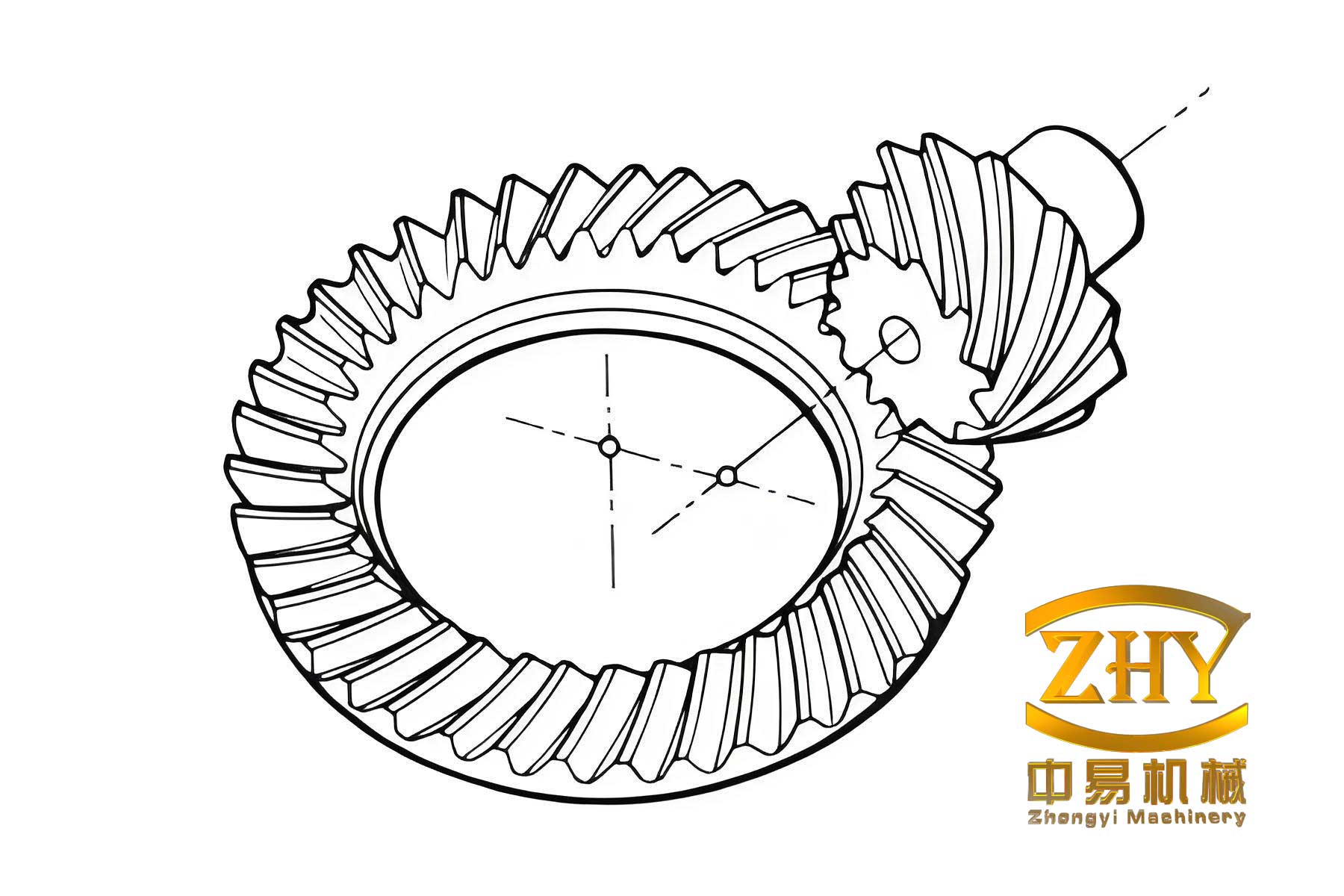
In the field of mechanical transmission, gearing systems play a fundamental role in power transfer and motion control across a wide range of industrial applications. Among the many gear types available to designers, hypoid gears hold a special position due to their unique geometric characteristics and superior transmission performance. Unlike conventional bevel gears, where the axes of the pinion and gear intersect, hypoid gears are designed with offset axes, which provides several distinct advantages in practical engineering applications. The offset arrangement enables a larger reduction ratio within a more compact envelope, smoother meshing action, and enhanced load-carrying capacity, making hypoid gears the preferred choice for automotive drive axles and various heavy-duty power transmission systems.
The geometric complexity of hypoid gears presents significant challenges in design, manufacturing, and quality control. Unlike standard involute gears, the tooth surfaces of hypoid gears are generated through complex manufacturing processes that involve specialized machine tools and cutting methods. The meshing quality of the gear pair, which directly influences performance parameters such as noise, vibration, load distribution, and fatigue life, is difficult to predict and control with precision. Traditional empirical approaches and trial-and-error methods are time-consuming, costly, and often fail to achieve the desired level of accuracy and reliability.
As China’s economy continues to develop rapidly, the demand for high-performance automotive vehicles and industrial machinery has increased substantially. This growing demand has highlighted the urgent need for advanced manufacturing technologies that can produce hypoid gears with consistent quality and superior performance. The domestic Chinese gear industry has long relied on technologies introduced from Gleason Works in the United States, but there is a pressing need for independent innovation in gear design and manufacturing to improve the reliability and competitiveness of Chinese-made gear products.
My research focuses on exploring new digital manufacturing methods for hypoid gears, with particular emphasis on modeling techniques and stress analysis approaches. The motivation for this work stems from several observed limitations in existing manufacturing practices:
First, the traditional design and calculation process for hypoid gears is extremely complex and computationally intensive. The determination of optimal machining parameters requires solving systems of nonlinear equations, iterative procedures, and careful consideration of numerous geometric constraints. This complexity often results in manufacturing parameters that are approximations rather than optimal solutions.
Second, conventional cutting-based manufacturing methods inherently damage the material microstructure near the tooth surface. The cutting process interrupts the continuous flow of metal fibers, leaves tool marks on the tooth surfaces, and creates stress concentration at the root fillet region. These factors significantly reduce the load-carrying capacity and fatigue life of the gear pair, particularly under high-speed and heavy-load operating conditions encountered in automotive applications.
Third, the optimization of the tooth root transition region, which is critical for reducing bending stress and improving fatigue strength, is constrained by the geometric limitations of conventional cutting tools and machine tool structures. The flexibility to optimize this region is severely limited when traditional manufacturing methods are employed.
Fourth, achieving precise three-dimensional solid models of hypoid gears that accurately represent the actual tooth geometry, including the complex root transition surface, remains a challenging task. Such models are essential for finite element analysis, virtual assembly simulation, and the verification of machining results.
My research aims to address these limitations by proposing a comprehensive approach that combines theoretical analysis, computational modeling, and experimental validation. The specific objectives of this work are as follows: to develop a systematic methodology for the digital manufacturing modeling of hypoid gears, to investigate new methods for tooth surface modification based on conjugate gear theory, and to analyze the stress distribution in the tooth root transition region under various loading conditions.
The remainder of this article is organized as follows: Chapter 2 introduces the fundamental machining methods for hypoid gears and establishes the theoretical foundation of the local synthesis method. Chapter 3 presents the detailed calculation procedure for gear geometric parameters and machining parameters. Chapter 4 focuses on the precise three-dimensional modeling approach and finite element stress analysis of the gear pair. Chapter 5 describes the novel tooth surface modification technique based on fully conjugated tooth surfaces. Finally, Chapter 6 summarizes the key findings and conclusions of this research.
2. Fundamental Machining Methods for Hypoid Gears
2.1 Classification of Machining Methods
In the manufacturing practice of hypoid gears, a variety of machining methods have been developed and refined over the decades. These methods can be broadly classified into two categories based on the fundamental machining principle: form cutting (also known as forming) and generating cutting (also known as roll-cutting or hobbing).
The form cutting method, referred to as the Formate method in the Gleason system, is particularly well-suited for machining the gear member of hypoid gears with relatively large pitch angles. In this method, the tooth profile of the gear is essentially the reverse of the cutter blade profile, with the cutter blades directly plunge-cutting into the workpiece. The gear member, which is typically the larger of the two mating gears, is processed using this efficient method since its tooth surfaces closely match the shape of the cutting tools. The Formate process offers significant advantages in terms of productivity and is widely adopted in mass production applications such as automotive manufacturing. For gear pitch angles greater than 45 degrees, the application of form cutting with straight-sided cutter blades is appropriate for rough cutting. When the gear pitch angle exceeds 70 degrees, this method can be used for finish cutting as well. Additional variations of the form cutting technique include the use of circular broach cutters and the Helixform method, which involves a reciprocating axial motion of the cutter head to produce theoretically correct conjugation.
The generating method, also known as the Generated or roll-cutting method, is based on the fundamental principle that the tooth surface is generated as the envelope of a series of cutter blade positions as the workpiece and cutter rotate in a synchronized manner. This method is commonly used for machining the pinion member and can be further classified into several variants:
| Method | Description | Application |
|---|---|---|
| Single-Side Cutting | Both tooth flanks of a gap are machined together during roughing; during finish cutting, the two sides of the pinion are cut separately with different cutter settings | General-purpose machining with flexible adjustment |
| Double-Side Cutting | Both sides of a tooth gap are machined simultaneously using a double-side cutter; several sub-variants exist including single-machine and fixed-setting arrangements | High-volume production of gear and pinion |
| Double Helical Method | Both pinion and gear are cut using double-side cutters, with all tooth gaps machined in a single continuous operation | Ultra-high-volume production |
In practice, the most commonly used designations for machining methods used for hypoid gears are three-letter codes that specify both the gear and pinion machining operations. For example:
- HGM: Hypoid gear with Generated gear member and Modified-roll pinion
- HFT: Hypoid gear with Formate gear member and Tilt-type pinion
- SGM: Spiral bevel gear with Generated gear member and Modified-roll pinion
- SFT: Spiral bevel gear with Formate gear member and Tilt-type pinion
In the HFT method, the gear is produced using the form cutting process, while the pinion is generated using a tilted cutter head. The tilt mechanism allows the cutter axis to be inclined relative to the cradle axis, creating the necessary pressure angle modifications on the pinion tooth surfaces to achieve proper meshing with the form-cut gear.
2.2 Fundamentals of the Local Synthesis Method
The local synthesis method, originally developed by F.L. Litvin in the 1960s and subsequently refined in collaboration with Y. Gutman in the 1980s, provides a systematic framework for determining the optimal machine-tool settings for machining the pinion of hypoid gears or spiral bevel gears. The fundamental principle underlying this approach is to control the local geometric properties of the contacting tooth surfaces at a reference point located at the center of the desired contact pattern.
The basic concept is elegantly simple: rather than aiming for the theoretically ideal line contact between the mating tooth surfaces, which is extremely sensitive to manufacturing and assembly errors, the local synthesis method deliberately introduces a controlled amount of mismatch. This mismatch results in point contact between the tooth surfaces in the unloaded state, which expands into an elliptical contact zone under load due to elastic deformation of the gear teeth. The location and orientation of this contact ellipse, the transmission error function, and the path of contact can all be influenced by adjusting the machine-tool parameters.
The complete local synthesis procedure proceeds through the following steps:
- Determine gear machining parameters. For the Formate gear, the machining parameters are relatively straightforward to establish since the gear tooth surfaces are direct copies of the cutter blade profiles. The key parameters include the cutter radius, blade angles, machine root angle, and the radial and angular cutter positions.
- Compute the gear tooth surface. The three-dimensional coordinates of the gear tooth surface are calculated using the geometric relationships between the cutter coordinate system, the machine coordinate system, and the gear coordinate system.
- Select a reference point. A reference point M is selected on the gear tooth surface, typically at the center of the intended contact pattern. The position is usually chosen at the midpoint of the tooth flank in the lengthwise direction and at a predetermined height along the tooth profile.
- Calculate principal curvatures. At the reference point, the principal curvatures and principal directions of the gear tooth surface are determined using differential geometry.
- Prescribe local synthesis parameters. The following conditions are prescribed at the reference point:
- The first derivative of the transmission ratio function \( m’_{21} \), which controls the amount of parabolic transmission error
- The tangent direction of the contact path on the gear tooth surface, characterized by the angle \( \eta_2 \)
- The semi-major axis length \( a \) of the instantaneous contact ellipse
- Compute pinion principal curvatures. Using the fundamental equations of tooth surface contact, the required principal curvatures and principal directions of the pinion tooth surface at the reference point are calculated to satisfy the prescribed synthesis parameters.
- Determine machine-tool settings. From the calculated principal curvatures of the pinion tooth surface, all necessary machine-tool settings are determined, including the cutter radius, blade angles, cradle angle, radial setting, vertical offset, axial setting, sliding base, tilt angle, swivel angle, and roll ratio.
2.3 Fundamental Equations of Tooth Surface Contact
At the contact point M of two mating tooth surfaces \( \Sigma_1 \) and \( \Sigma_2 \), the following fundamental relationships must be satisfied:
The relative velocity vector at the contact point can be expressed as:
\[
\vec{v}^{(12)} = \vec{\omega}^{(1)} \times \vec{r}^{(1)} – \vec{\omega}^{(2)} \times \vec{R}
\]
where \( \vec{\omega}^{(i)} \) is the angular velocity vector of gear \( i \), \( \vec{r}^{(1)} \) is the position vector from the rotation axis of gear 1 to the contact point, and \( \vec{R} \) is the vector separating the axes of rotation of the two gears.
At the point of tangency of the two tooth surfaces, the relative velocity lies in the common tangent plane, and the fundamental relationship known as the equation of meshing applies:
\[
\vec{n} \cdot \vec{v}^{(12)} = 0
\]
where \( \vec{n} \) is the common unit normal vector at the contact point.
The basic system of equations, known as the Litvin equations, relates the principal curvatures and principal directions of the two contacting surfaces at the instantaneous contact point. Let us denote:
| Symbol | Meaning |
|---|---|
| \( \vec{e}_f, \vec{e}_h \) | Unit vectors of the principal directions on surface \( \Sigma_1 \) |
| \( k_f, k_h \) | Principal curvatures of surface \( \Sigma_1 \) corresponding to \( \vec{e}_f, \vec{e}_h \) |
| \( \vec{e}_s, \vec{e}_q \) | Unit vectors of the principal directions on surface \( \Sigma_2 \) |
| \( k_s, k_q \) | Principal curvatures of surface \( \Sigma_2 \) corresponding to \( \vec{e}_s, \vec{e}_q \) |
| \( \sigma^{(12)} \) | Angle between \( \vec{e}_f \) and \( \vec{e}_s \) |
The linear system of equations can be written as:
\[
a_{11} v_s^{(1)} + a_{12} v_q^{(1)} = a_{13} \tag{1}
\]
\[
a_{21} v_s^{(1)} + a_{22} v_q^{(1)} = a_{23} \tag{2}
\]
\[
a_{31} v_s^{(1)} + a_{32} v_q^{(1)} = a_{33} \tag{3}
\]
where the coefficients \( a_{ij} \) are given by:
\[
a_{11} = k_f \cos^2 \sigma^{(12)} + k_h \sin^2 \sigma^{(12)} – k_s
\]
\[
a_{12} = a_{21} = 0.5 \sin(2\sigma^{(12)})(k_h – k_f)
\]
\[
a_{22} = k_f \sin^2 \sigma^{(12)} + k_h \cos^2 \sigma^{(12)} – k_q
\]
\[
a_{13} = \vec{\omega}^{(12)} \cdot \vec{e}_h – \vec{v}_{tr}^{(1)} \cdot (\vec{n} \times \vec{e}_s) – \vec{v}_{tr}^{(2)} \cdot (\vec{n} \times \vec{e}_q)
\]
For line contact, the coefficient matrix A must be singular, requiring that \( \det(A) = 0 \), which yields the compatibility conditions for the principal curvatures and directions of the two surfaces in continuous line contact.
For point contact, the solution is unique. The equations are supplemented with the prescribed local synthesis parameters to obtain the required pinion curvatures.
2.4 Prescribed Parameters in Local Synthesis
First derivative of transmission ratio. The transmission error function can be approximated as a parabolic function in the vicinity of the reference point. The parameter \( m’_{21} \) controls the coefficient of the quadratic term. For hypoid gears with a concave transmission error curve (which is desirable for smooth engagement), the following condition applies:
\[
\delta(\phi_1) = -\frac{1}{2} m’_{21} (\phi_1 – \phi_1^{(0)})^2
\]
The negative value of \( m’_{21} \) produces a downward-opening parabola, meaning the actual rotation angle of the gear lags the theoretical value during approach and recess.
Tangent direction of contact path. The angle \( \eta_2 \) determines the direction of the contact path on the gear tooth surface. Together with the relative velocity components, this parameter influences the direction of the contact trace. For the conventional case where the gear is right-handed and the pinion is left-handed:
- For the drive side (gear convex flank, pinion concave flank): \( \eta_2 \) in the range of 0° to 90°
- For the coast side (gear concave flank, pinion convex flank): \( \eta_2 \) in the range of 90° to 180°
Semi-major axis of contact ellipse. The contact ellipse dimensions can be estimated from the relative principal curvatures and the elastic deformation of the contacting bodies. The relationship involves the curvature parameters through the following expression:
\[
\frac{a}{b} = \frac{2\sqrt{A} – \sqrt{A^2 – B^2}}{2\sqrt{A} + \sqrt{A^2 – B^2}}
\]
where \( A \) and \( B \) are combinations of the principal curvatures of the two contacting surfaces at the contact point.
3. Calculation of Geometric Parameters and Machining Parameters
3.1 Geometric Design of Hypoid Gear Pairs
The geometric design of a hypoid gears pair begins with the specification of basic parameters such as the shaft angle \( \Sigma \), the number of teeth on the pinion \( z_1 \) and gear \( z_2 \), the direction of spiral, and the offset distance E. In my research, I consider a hypoid gear pair with the following characteristics:
| Parameter | Pinion | Gear |
|---|---|---|
| Number of teeth | 10 | 41 |
| Shaft angle (°) | 90 | |
| Spiral direction | Left | Right |
| Offset distance (mm) | 31.8 | |
| Pressure angle (°), convex flank | 24 | 20 |
| Pressure angle (°), concave flank | 17 | 18 |
| Mean spiral angle (°) | 50 | 29 |
| Outer cone distance (mm) | 117.2 | 101.3 |
| Outside diameter (mm) | 78.4 | 195.2 |
| Addendum (mm) | 7.3 | 1.5 |
| Dedendum (mm) | 2.3 | 8.3 |
| Whole tooth height (mm) | 9.6 | 9.8 |
| Pitch angle (°) | 15.5 | 73.7 |
| Face angle (°) | 20.5 | 74.8 |
| Root angle (°) | 14.2 | 68.1 |
The pitch angle of the gear member, \( \delta_2 \), the pinion spiral angle \( \beta_1 \), and the shell-angle offset \( \eta \), determine the location of the pitch point. The gear pitch radius at the midpoint is given by:
\[
r_2 = \frac{1}{2}(d_2 – b_2 \sin \delta_2)
\]
where \( d_2 \) and \( b_2 \) are the outer pitch diameter and face width of the gear, respectively. The pitch point location is iteratively adjusted until convergence is achieved with respect to the cutter radius.
For the iterative procedure, I implemented the calculation in the VC++ programming environment to automate the computations and ensure numerical accuracy. The input parameters include the gear pitch angle, pinion spiral angle, cutter radius, and several other key dimensions. The iterative process adjusts the shell-angle offset until the calculated limiting normal radius of curvature matches the selected cutter radius within a specified tolerance.
Once the pitch cone parameters are established, the remaining blank dimensions can be determined systematically. The addendum and dedendum at the midpoint are calculated based on the desired strength and clearance requirements. The face angle and root angle are then determined using either standard or Duplex taper contraction methods. The resulting blank dimensions provide the basis for generating the three-dimensional models of the gear blanks.
3.2 Machining Parameters for the Formate Gear
For the Formate gear, the cutting process is carried out on a gear cutting machine such as the No. 607. The gear is generated with both tooth flanks cut simultaneously using a double-side cutter. The machining setup is characterized by the following key parameters:
The blade profile for the gear cutter is defined by the following equations in the cutter coordinate system:
\[
\vec{r}_G(u_G, \theta_G) = \begin{bmatrix} (r_G + u_G \sin \alpha_2) \cos \theta_G \\ (r_G + u_G \sin \alpha_2) \sin \theta_G \\ -u_G \cos \alpha_2 \\ 1 \end{bmatrix}
\]
where \( r_G \) is the cutter radius, \( u_G \) and \( \theta_G \) are the surface coordinates, and \( \alpha_2 \) is the blade pressure angle. The corresponding unit normal vector is:
\[
\vec{n}_G = \begin{bmatrix} \cos \alpha_2 \cos \theta_G \\ \cos \alpha_2 \sin \theta_G \\ -\sin \alpha_2 \end{bmatrix}
\]
After transforming the cutter surface into the gear coordinate system through the machine coordinate system, the gear tooth surface can be expressed as:
\[
\vec{r}_2(u_G, \theta_G) = M_{2m} M_{mG} \vec{r}_G(u_G, \theta_G)
\]
where the transformation matrices \( M_{mG} \) and \( M_{2m} \) account for the radial cutter position, angular cutter position, machine root angle, and axial setting.
The machining parameters for the gear, calculated based on the Gleason calculation procedure, are summarized in Table 3:
| Parameter | Value |
|---|---|
| Radial cutter position (mm) | 93.2 |
| Angular cutter position (°) | 63.8 |
| Machine root angle (°) | 68.2 |
| Mounting distance (mm) | 56.1 |
| Outside blade angle (°) | 24 |
| Inside blade angle (°) | 17 |
| Cutter radius (mm) | 95.2 |
| Blade point width (mm) | 2.3 |
| Blade tip radius (mm) | 1.016 |
3.3 The Local Synthesis Procedure for Pinion Machining
The pinion machining parameters are determined based on the local synthesis method. The procedure involves several stages, beginning with the calculation of the gear tooth surface and its principal curvatures at the reference point, followed by the application of the local synthesis equations to determine the required pinion tooth surface curvature characteristics.
Since the gear is manufactured by the Formate method, the gear tooth surface is a direct copy of the cutter surface. The principal curvatures at the reference point can be obtained from the cutter geometry:
\[
k_s^{(2)} = \frac{\cos \alpha_2}{r_G + u_G \sin \alpha_2}, \quad k_q^{(2)} = 0
\]
The principal directions on the gear tooth surface are aligned with the cutter blade profile and the direction of the cutter rotation.
Using the coordinate transformation from the gear coordinate system to the meshing coordinate system, the gear tooth surface, normal vector, and principal directions can be expressed in the fixed coordinate system associated with the gear housing:
\[
\vec{r}_h^{(2)}(\theta_G, u_G) = M_{hd} M_{d2} \vec{r}_2(\theta_G, u_G)
\]
The meshing equation at the reference point is:
\[
\vec{n}_h^{(2)} \cdot \vec{v}_h^{(12)} = 0
\]
where the relative velocity is computed considering both the gear and pinion angular velocity vectors:
\[
\vec{v}_h^{(12)} = \vec{\omega}_h^{(1)} \times \vec{r}_h – \vec{\omega}_h^{(2)} \times (\vec{r}_h – \vec{E})
\]
From the meshing equation, the rotational position of the gear at the reference point can be determined. Once the gear tooth surface and its properties at the reference point are established, the local synthesis parameters are prescribed:
- \( m’_{21} \): The derivative of the transmission ratio with respect to pinion rotation angle
- \( \eta_2 \): The angle between the tangent to the contact path and the principal direction \( s \) on the gear tooth surface
- \( a \): The semi-major axis of the instantaneous contact ellipse
Using the fundamental equations of tooth surface contact developed in Chapter 2, the principal curvatures and principal directions of the pinion tooth surface at the reference point can be solved. The computed results are then used to determine the pinion machining parameters through the following steps:
3.3.1 Determination of Cutter Radius for the Pinion
The cutter radius for the pinion is calculated using the condition that the cutter tooth surface and the pinion tooth surface must be in line contact during the machining process. The equation relating the cutter curvature to the pinion curvature is:
\[
k_f^{(p)} = a_{22} \cos^2 \sigma^{(1p)} + 2a_{12} \sin \sigma^{(1p)} + a_{11} \sin^2 \sigma^{(1p)}
\]
The pinion cutter radius is then:
\[
r_p = \frac{\cos \alpha_1}{k_f^{(p)}} – u_p \sin \alpha_1
\]
3.3.2 Determination of Roll Ratio
The roll ratio determines the relationship between the cradle rotation and the workpiece rotation. At the reference point, the relative velocity components are determined from the basic equations, and the machine roll is calculated as:
\[
R_{1p} = m_{1p}^{(c)}
\]
3.3.3 Determination of Machine Settings
The remaining machine settings include the vertical offset, axial setting, sliding base, radial cutter position, angular cutter position, tilt angle, and swivel angle. The vertical offset E is calculated as:
\[
E = \frac{Y_c^{(p)} – m_{1p}^{(c)} v_{trx}^{(p)}}{m_{1p}^{(c)}}
\]
The axial setting and sliding base are determined from the spatial position of the pinion reference point and the machine root angle:
\[
X_{1G} = \frac{X_c^{(p)} – m_{1p}^{(c)} v_{try}^{(p)}}{\cos \gamma_1}
\]
The machine settings for the pinion, calculated for the example case, are summarized in Table 4:
| Parameter | Concave flank | Convex flank |
|---|---|---|
| Cradle angle (°) | 147.1 | 153.3 |
| Radial cutter position (mm) | 97.9 | 92.5 |
| Machine root angle (°) | 355.6 | 355.7 |
| Tilt angle (°) | 78.4 | 90.8 |
| Swivel angle (°) | 241.2 | 221.3 |
| Roll ratio | 4.03 | 3.87 |
| Blade angle (°) | 14 | 31 |
| Cutter radius (mm) | 92.5 | 97.9 |
| Blade tip radius (mm) | 0.635 | 0.635 |
For the calculation of these parameters, I utilized the MATLAB software environment to implement the complex iterative procedures. The computation of the principal curvatures, the assembly of the fundamental equations, and the solution of the nonlinear system of equations all require a robust and numerically stable approach.
4. Digital Modeling and Stress Analysis of Hypoid Gears
4.1 Mathematical Model of the Gear Tooth Surface with Root Fillet
The accurate three-dimensional modeling of hypoid gears requires the consideration of not only the working tooth surface but also the root transition surface. In my research, I employed a specialized cutter blade profile with a rounded tip corner, which improves the bending strength and fatigue resistance of the gear teeth compared to sharp-edged blades.
The cutting blade profile for the gear comprises two distinct segments: a straight line segment that generates the working portion of the tooth flank, and a circular arc segment that generates the root transition region. The working tooth surface equation can be expressed as:
\[
\vec{r}_G(u_G, \theta_G) = \begin{bmatrix} (r_G \pm u_G \sin \alpha_2) \cos \theta_G \\ (r_G \pm u_G \sin \alpha_2) \sin \theta_G \\ -u_G \cos \alpha_2 \\ 1 \end{bmatrix}
\]
where the upper sign corresponds to the outside blade and the lower sign to the inside blade.
The transition surface equation is:
\[
\vec{r}_G'(\beta, \theta_G) = \begin{bmatrix} (r_G – r_0 + u_{G0}\sin\alpha_2 + r_0\cos\beta)\cos\theta_G \\ (r_G – r_0 + u_{G0}\sin\alpha_2 + r_0\cos\beta)\sin\theta_G \\ -u_{G0}\cos\alpha_2 \pm r_0(1-\sin\beta) \\ 1 \end{bmatrix}
\]
The parameter \( u_{G0} \) determines the boundary between the working surface and the transition surface, and its value depends on the blade tip radius.
4.2 Calculation of Gear Tooth Surface Points
Since the gear is manufactured using the Formate method, the tooth surface is a direct copy of the cutter surface. Therefore, the discretization of the gear tooth surface is accomplished by varying the surface parameters \( u_G \) and \( \theta_G \) through their respective ranges.
The range of \( u_G \) is determined by the whole tooth height \( h_2 \) and the blade angle \( \alpha_2 \):
\[
0 \leq u_G \leq \frac{h_2}{\cos \alpha_2}
\]
The range of \( \theta_G \) is approximated based on the face width of the gear:
\[
\theta_G \approx \frac{b_2}{r_G}
\]
To ensure sufficient coverage of the tooth surface, I set the range of \( \theta_G \) slightly larger than this approximation. The discrete points are then calculated using a double-loop iteration within the MATLAB programming environment.
4.3 Calculation of Pinion Tooth Surface Points
Unlike the gear, the pinion tooth surface is generated through the generating process. The pinion tooth surface is the envelope of the cutter blade surface during the generating motion. Moreover, the pinion is characterized by a special geometric feature consisting of a protruding portion (the so-called “protuberance” or “protuberance flank”) and a root fillet region.
To calculate the pinion tooth surface points, I employed the tooth surface rotation-projection principle. According to this principle, a rotating projection plane is defined such that a point on the gear tooth surface with coordinates \( (x, y, z) \) corresponds to a point \( (X, Y) \) on the projection plane through the mapping:
\[
X = x, \quad Y = \sqrt{y^2 + z^2}
\]
The tooth surface is divided into a grid of 5×9 points in the lengthwise and profile directions, respectively. For the working tooth surface, the upper boundary is the tooth top line and the lower boundary is the intersection line between the working surface and the protuberance flank. The protuberance flank is bounded by the intersection with the working surface on one side and the intersection with the root transition surface on the other. The root transition surface extends from its intersection with the protuberance flank to the root line.
For the pinion, I used a blade profile with a protuberance to avoid interference between the pinion root and the gear tooth tip. The protuberance flank equation is:
\[
\vec{r}_f^b(u_f, \theta_P) = \begin{bmatrix} (r_f \pm u_f \sin \alpha_1) \cos \theta_P \\ (r_f \pm u_f \sin \alpha_1) \sin \theta_P \\ -u_f \cos \alpha_1 \\ 1 \end{bmatrix}
\]
The root transition surface equation for the pinion is:
\[
\vec{r}_f^c(\lambda_f, \theta_P) = \begin{bmatrix} (x_f \pm \rho_f \sin \lambda_f) \cos \theta_P \\ (x_f \pm \rho_f \sin \lambda_f) \sin \theta_P \\ -\rho_f(1-\cos \lambda_f) \\ 1 \end{bmatrix}
\]
with the relationship \( x_f = r_f \pm \rho_f (1 – \sin \alpha_f)/\cos \alpha_f \).
Using the rotation-projection method, the three-dimensional coordinates of the pinion tooth surface can be calculated by solving the nonlinear system of equations formed by the surface equations and the projection relationships.
4.4 Three-Dimensional Solid Modeling
The process of generating the three-dimensional model of the hypoid gears was accomplished through the following steps:
- Data preparation. The calculated three-dimensional discrete points are saved in the .DTA format recognized by the UG NX software.
- Surface construction. The discrete points are imported into UG NX, and the tooth surface is constructed using the Through Curves Surface or similar surface generation techniques.
- Blank modeling. The gear blank is created using the rotational modeling features, based on the calculated blank dimensions including the pitch angle, face angle, root angle, outer cone distance, and face width.
- Tooth space generation. The tooth surface patches are extended and stitched to form a closed volume. The intersection of this volume with the gear blank creates a single tooth space.
- Pattern generation. The tooth space is arrayed around the rotational axis to create the complete gear with the desired number of teeth.
- Assembly. The pinion and gear models are assembled by applying distance and alignment constraints to reproduce the correct shaft angle and offset distance.
Figure 4 shows the three-dimensional model of the pinion and the assembled gear pair, respectively. The solid model accurately represents the tooth geometry including the root fillet region, the protuberance detail, and the transition surfaces.
4.5 Finite Element Analysis of the Gear Pair
For the finite element analysis of the hypoid gears pair, I adopted a strategy that balances computational efficiency with numerical accuracy. The finite element model includes three teeth from each member of the gear pair, which is sufficient to capture the contact behavior while limiting the total number of elements and nodes.
The complete solid models were transferred to HyperMesh for mesh generation. The mesh was created using free tetrahedral elements with a target element size of 1 mm and a minimum element size of 0.3 mm. The curvature and proximity refinement features of HyperMesh were utilized to automatically refine the mesh in regions of high geometric complexity, such as the root fillet region and the contact area. This ensures adequate accuracy in the regions where stress concentration is expected.
After mesh generation, the model was transferred to ANSYS for the loading contact analysis. The boundary conditions were imposed as follows:
- The gear was fully constrained in all six degrees of freedom.
- The pinion was allowed to rotate about its own axis, with all other degrees of freedom constrained.
- Torque values of 500 N·m and 1000 N·m were applied to the pinion in the direction that maintains contact between the pinion concave flank and the gear convex flank.
To simulate the complete meshing cycle, five distinct positions representing different phases of engagement were analyzed separately. For each position, the gear pair was rotated to bring the corresponding tooth pair into contact, and the loading conditions were re-applied.
4.5.1 Results of Contact Stress Analysis
The contact stress distribution obtained from the finite element analysis exhibits several notable features. At each load level, the maximum contact stress occurs at the point where the contact ellipse is centered, and the stress decreases gradually in all directions from this point. The stress distribution pattern on the gear flank shows a clear progression as the meshing cycle advances.
The contact stress levels at the torque of 1000 N·m are significantly higher than those at 500 N·m, as expected from the linear relationship between applied load and contact stress. A key observation is that the maximum stress position traverses from the toe of the tooth toward the heel, and from the top of the tooth profile toward the root as the meshing progresses.
The numerical results verified the accuracy of the three-dimensional model and confirmed that the tooth surface point calculations were properly executed. The smooth stress distribution throughout the contact zone indicates that the meshing surfaces are geometrically compatible.
4.5.2 Root Bending Stress Analysis
The root bending stress analysis revealed the beneficial effects of maintaining a correctly designed tooth root transition surface. The presence of the root fillet radius allows stresses in the transition region to be distributed more uniformly, reducing the sharp stress concentration that would occur at the sharp intersection between the root surface and the tooth flank.
At each load level, the maximum bending stress occurs in the root region on the tension side of the tooth, which is the side opposite to the contact point. The stress gradient from the maximum stress location toward the interior of the tooth is relatively smooth, confirming the effectiveness of the transition surface design in mitigating stress concentration.
5. Tooth Surface Modification Based on Conjugate Gear Theory
5.1 Calculation of the Fully Conjugated Pinion Tooth Surface
Traditional methods for determining the pinion machining parameters of hypoid gears rely on the local synthesis technique, which involves complex iterative calculations and numerical procedures. The accuracy of the resulting machining parameters depends on many factors, and the final tooth surface geometry may deviate from the theoretical design within acceptable but non-negligible tolerances. Moreover, the conventional machining process restricts the flexibility in optimizing the root transition region due to the physical constraints of the cutting tools and the machine tool structure.
In this chapter, I present an alternative approach that entirely bypasses the calculation of pinion machining parameters. The fundamental concept is elegant: Since the gear tooth surface is known (and can be precisely manufactured), the pinion tooth surface can be calculated directly from gear tooth surface using the principle of conjugate gear theory. This approach, while conceptually straightforward, requires careful numerical implementation to ensure accuracy and stability.
The calculation procedure begins with the gear tooth surface equations in the gear coordinate system S2. The gear tooth surface and normal vector are transformed to the housing-fixed coordinate system Sh using the two coordinate transformation matrices:
\[
\vec{r}_h^{(2)}(\theta_G, u_G, \phi_2) = M_{hd} M_{d2}(\phi_2) \vec{r}_2(\theta_G, u_G)
\]
where \( M_{d2} \) represents the rotation of the gear about its own axis and includes the angular parameter \( \phi_2 \).
The meshing equation, which must be satisfied during the entire meshing cycle, can be expressed as:
\[
\vec{n}_h \cdot \vec{v}_h^{(12)} = 0
\]
Expanding the vectors into their components and simplifying, the meshing equation reduces to a trigonometric equation in the gear rotation angle \( \phi_2 \):
\[
A \sin \phi_2 + B \cos \phi_2 = C
\]
The coefficients A, B, and C are functions of the gear tooth surface parameters \( u_G \) and \( \theta_G \). The solution for \( \phi_2 \) is:
\[
\phi_2 = \arcsin\left(\frac{C}{\sqrt{A^2 + B^2}}\right) – \arctan\left(\frac{B}{A}\right)
\]
Thus, for each pair of surface parameters \( (u_G, \theta_G) \), the corresponding gear rotation angle \( \phi_2 \) at the meshing instant can be determined. From the meshing condition and the known rotation ratio:
\[
\frac{\phi_2}{\phi_1} = \frac{z_1}{z_2}
\]
the pinion rotation angle is obtained. The pinion tooth surface is then calculated by transforming the gear tooth surface points into the pinion coordinate system:
\[
\vec{r}_1(\theta_G, u_G) = M_{1h} M_{hd} M_{d2}(\phi_2) \vec{r}_2(\theta_G, u_G)
\]
This calculation must be repeated for a sufficiently dense grid of points to provide an accurate representation of the fully conjugated pinion tooth surface. The resulting pinion tooth surface, if manufactured and assembled with the gear under perfectly rigid and error-free conditions, would produce line contact with zero transmission error.
In practice, however, such a fully conjugated pinion is not suitable for real-world applications. The high sensitivity of the line contact configuration to manufacturing and assembly errors leads to edge loading and high stress concentrations. Therefore, the fully conjugated pinion must be modified to achieve localized contact and a controlled transmission error profile through the contact region.
5.2 Parabolic Modification of the Conjugated Pinion Tooth Surface
The modification of the fully conjugated pinion tooth surface is accomplished through a systematic procedure that introduces controlled deviations from the theoretical conjugate surface. I selected a parabolic modification law due to its simplicity, smoothness, and verifiable results. The modification is applied in two directions: along the tooth length direction (corresponding to the face width coordinate) and along the tooth height direction (corresponding to the profile coordinate).
To implement the modification, I established a modification coordinate system Sm whose origin is located at the intersection of the pitch cone line and the mid-face width line of the pinion. The Xm axis lies along the pitch cone line, the Ym axis coincides with the normal to the tooth surface at the reference point, and the Zm axis is perpendicular to the pitch cone generating line.
In the tooth length direction, the parabolic modification amount is given by:
\[
\Delta y_m = a_m x_m^2
\]
At the two ends of the tooth face width, the prescribed modification amount is specified. This determines the coefficient \( a_m \) from:
\[
a_m = \frac{\Delta y_{max}}{(b_1/2)^2}
\]
where \( b_1 \) is the pinion face width and \( \Delta y_{max} \) is the maximum modification offset at the tooth ends.
Similarly, in the tooth height direction, the parabolic modification is:
\[
\Delta y_m = b_m z_m^2
\]
The coefficient \( b_m \) is determined by the prescribed modification amount at the tooth top addendum.
For each grid point on the fully conjugated pinion tooth surface, the total modification amount is calculated by combining the contributions from both directions:
\[
\Delta r = \sqrt{(\Delta y_{m,i})^2 + (\Delta y_{m,j})^2}
\]
where index \( i \) corresponds to the face width position and index \( j \) corresponds to the profile position. The modified pinion tooth surface coordinates are then computed by shifting the original points along the normal direction by the calculated modification amount.
For the example case with gear pair \( z_1 = 26, z_2 = 35 \), I prescribed a maximum modification of 0.10 mm in the lengthwise direction and 0.03 mm in the profile direction. After modification, the assembled gear pair exhibits a localized contact pattern as expected from theoretical considerations.
5.3 Root Transition Surface Optimization
One of the significant advantages of the new manufacturing method is the flexibility to optimize the root transition surface without the geometric constraints imposed by conventional cutting tools. In the conventional machining process, the root filler radius is determined by the blade tip radius at the cutter, which must also satisfy other cutting-related constraints.
In the new approach, since the pinion tooth surface is first calculated and then modified, the root transition surface can be specified independently to achieve the optimal bending stress distribution. By increasing the root filler radius to the maximum permissible value that does not cause interference with the mating gear, the tooth root bending stress can be significantly reduced.
5.4 Experimental Validation of the Modified Pinion
To validate the theoretical predictions of the conjugate gear modification approach, I conducted experimental cutting tests and subsequent tooth surface measurements. The experimental procedure involved the following stages:
5.4.1 Pinion Cutting on a Machining Center
Given the specific characteristics of the proposed method, the pinion was machined on an FMH-630 four-axis CNC machining center. The machine parameters are:
| Parameter | Value |
|---|---|
| X-axis travel (mm) | 1000 |
| Y-axis travel (mm) | 850 |
| Z-axis travel (mm) | 850 |
| Rapid feed rate (mm/min) | 2400 |
| Spindle motor power (kW) | 18.5 |
| Maximum spindle speed (r/min) | 8000 |
| Cutting feed rate range (mm/min) | 1–8000 |
The pinion was machined from 45 steel. Before machining, the mounting fixture was checked for accuracy, with the end face runout at 0.01 mm and the outer diameter radial runout at 0.015 mm. The tool path was programmed based on the three-dimensional model generated in the UG software and verified for collisions or interferences before sending to the machine.
The machining process was executed in two stages: rough machining using an R3 ball-end mill and finish machining using an R2 ball-end mill. During finish machining, the concave and convex flanks of the pinion and the root transition surface were machined separately. The resulting pinion exhibited a smooth tooth surface finish, a well-formed transition between the tooth flank and the root surface, and an overall geometry consistent with the design intent.
5.4.2 Tooth Surface Measurement
The precision of the manufactured pinion surface was assessed using the JD45+ gear measuring center. The four-axis coordinate-measuring machine, equipped with a 2 mm diameter spherical stylus, was used to measure the pinion tooth surfaces in a point grid of 5×9 points. The measurement process involved:
- Setup: The pinion was aligned between upper and lower centers, with the grid points referenced from the tooth midpoint toward the toe and heel.
- Data acquisition: The coordinate data of each surface point were recorded for both tooth flanks.
- Analysis: The measured points were compared to the theoretical HFT-based pinion tooth surfaces, and the normal deviations were calculated.
The results of the tooth surface measurement are summarized as follows:
| Flank | Maximum Deviation (mm) | Location of Maximum Deviation |
|---|---|---|
| Concave flank | 0.0814 | Toe tip region |
| Convex flank | 0.0719 | Heel root region |
| Reference point | 0.000 | Contact center |
The deviations can be attributed to two primary sources. First, the numerical round-off and cumulative approximation errors inherent in the HFT parameter calculation process influence the theoretical reference surface. Second, machine tool positioning errors, tool deflection during the cutting process, and workpiece mounting misalignments contribute to the deviations between the measured and nominal geometry.
Overall, the measurement results confirmed that the pressure angles and spiral angles of the measured surface closely match the theoretical values. The deviation pattern is consistent, and the root mean square error falls within acceptable limits. The successful machining and measurement of the modified pinion tooth surface validate the feasibility and correctness of the complete conjugate modification theory.
6. Conclusions and Future Prospects
6.1 Summary of Findings
This research has systematically addressed the digital manufacturing modeling and stress analysis of hypoid gears, focusing on two distinct manufacturing scenarios: the conventional HFT-based method and a novel approach based on the modification of fully conjugated pinion tooth surfaces.
The key conclusions from this work are summarized below:
- I have developed a comprehensive procedure for calculating the geometric parameters and machining parameters of hypoid gears. The implementation in VC++ and MATLAB software environments enables automatic computation of the complex iterative calculations, reducing the risk of manual calculation errors and greatly improving the efficiency of the design process.
- I have established a precise three-dimensional modeling methodology for hypoid gears that includes the root transition surface. By properly representing the cutter blade geometry with a rounded tip and the protuberance, this modeling approach accurately reproduces the actual tooth surface geometry, including the previously neglected transition regions. This precise model forms the basis for accurate stress analysis and for the virtual verification of the gear pair before physical manufacturing.
- Through the combined use of MATLAB (for tooth surface point computation), UG (for solid modeling), HyperMesh (for mesh generation), and ANSYS (for finite element stress analysis), I have successfully implemented a loaded tooth contact analysis workflow for hypoid gears. The analysis results confirm the structural accuracy of the models and demonstrate the beneficial effect of the root transition surface in reducing tooth root bending stress and promoting a beneficial, uniform stress distribution in the root region.
- Based on the conjugate gear theory, I have developed a new method for calculating the pinion tooth surface directly from the gear tooth surface. This method eliminates the need for complex local synthesis calculations and provides a mathematically exact basis for tooth surface generation.
- I have proposed and implemented a parabolic tooth surface modification method applied to the fully conjugated pinion tooth surface. By modifying the tooth surface in both the lengthwise and profile directions, a localized contact pattern is achieved that is more tolerant to manufacturing and assembly variations while maintaining a controlled transmission error function.
- The new method provides significantly greater flexibility for optimizing the root transition surface compared to traditional machining processes. Since the pinion tooth surface geometry is not constrained by the cutter blade geometry and the machine tool structure, the root filler radius can be maximized to reduce bending stress and improve fatigue resistance.
- The cutting experiment on a four-axis machining center and the subsequent gear tooth measurement on the gear measuring center have validated the feasibility and precision of the proposed manufacturing method. The deviations between the measured tooth surface and the theoretical surface are within acceptable limits, confirming the correctness of the conjugated tooth surface modification theory.
6.2 Future Research Directions
While this research has achieved its stated objectives, several areas merit further investigation:
- Optimization of the numerical algorithms: The tooth surface point calculation relies on iterative methods that are sensitive to the initial guess. The development of more robust convergence techniques and the optimization of the iteration schemes would improve both computational speed and numerical stability.
- Elastic contact analysis: The current finite element analysis treated the gear teeth as rigid bodies in contact. Including elastic deformation of the gear body, bearing supports, and shaft structures would provide a more complete prediction of the actual contact stress and load distribution.
- Comprehensive experimental testing: Full-scale dynamic testing of the gear pair under varying load and speed conditions would provide valuable data for the quantitative validation of the finite element models and the overall gear performance.
- Alternative modification laws: While parabolic modification provides smooth contact transitions, other modification functions could potentially yield even better performance under specific operating conditions.
In summary, the research presented in this article has provided a new pathway for the digital manufacturing modeling of hypoid gears and has contributed to the ongoing efforts to improve the performance, reliability, and Fatigue strength of these critical machine elements.