
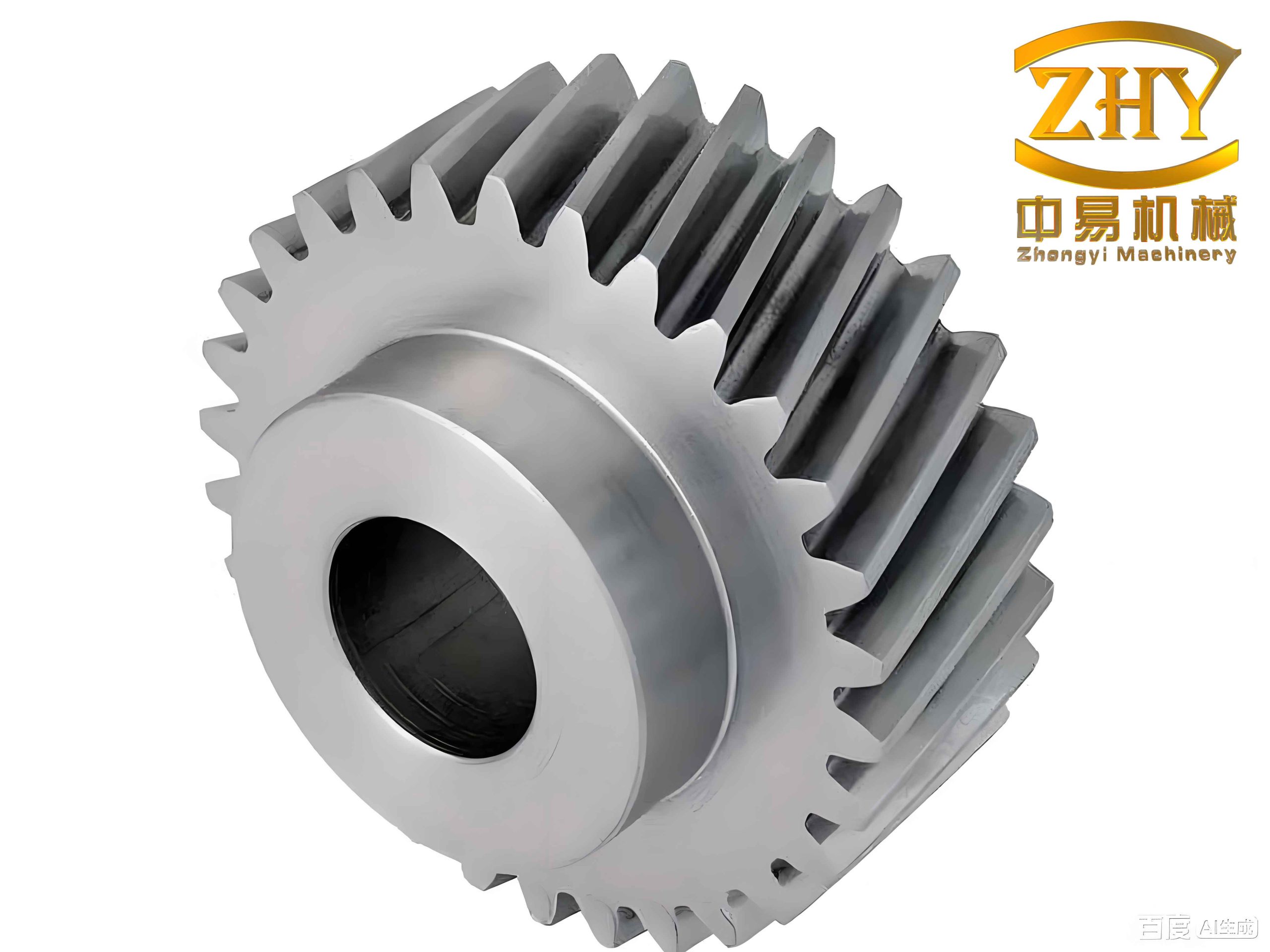
I focus on the dynamic transmission behavior of a high-speed helical gear meshing system because the helical gear is one of the most important power-transmission components in modern machinery. A high-speed helical gear pair can transfer large torque with smooth motion, high overlap ratio, and strong load capacity, but it also experiences strong internal and external excitations. These excitations include time-varying mesh stiffness, transmission error, backlash, eccentric unbalance, and input or output torque. If I model these effects with too few degrees of freedom, the predicted vibration of the helical gear system becomes incomplete, especially when the helical gear operates above 3000 rpm. Therefore, I construct a full-degree-of-freedom dynamic model for a shaft–helical gear pair–bearing transmission system and use it to study modal behavior, dynamic response, optimization, and tooth modification.
1. Motivation and Scope
I begin with the observation that a helical gear transmission system is not merely a pair of rotating disks. It is a coupled rotor system composed of flexible shafts, a helical gear pair, bearings, and supporting structures. The helical gear mesh introduces axial, transverse, torsional, and rotational coupling because the contact line is inclined by the helix angle. In a high-speed helical gear, the gyroscopic effect becomes important, and the unbalance force caused by eccentricity grows with the square of rotational speed. In addition, the mesh stiffness of a helical gear changes periodically as the contact line length changes, and the transmission error and backlash make the mesh force nonlinear. I therefore treat the helical gear pair as a twelve-degree-of-freedom substructure, with six degrees of freedom at each gear center, and I assemble it with Timoshenko beam elements and bearing elements.
My main purpose is to answer four questions. First, can a full-degree-of-freedom helical gear model reproduce the modal frequencies of a detailed finite element model while keeping the computation small enough for repeated dynamic analysis? Second, how do speed, mesh error, pressure angle, helix angle, eccentricity, and torque influence the vibration of the high-speed helical gear? Third, can I reduce the vibration of the helical gear system by optimizing eccentricity, pressure angle, and helix angle with a particle swarm algorithm? Fourth, after parameter optimization, can I further improve the helical gear transmission by tooth profile and lead modification, and can I verify the improvement through mesh error, loaded transmission error, equivalent stress, and fatigue life?
2. Full-Degree-of-Freedom Model of a High-Speed Helical Gear Transmission
I build the dynamic model in a substructure manner. The shaft is represented by Timoshenko beam elements, the helical gear pair is represented by a twelve-degree-of-freedom disk element, and the bearings are represented by stiffness and damping matrices. The structural damping is introduced through Rayleigh damping. After the element matrices are obtained, I assemble them in the same way as in finite element analysis. This gives a global dynamic equation for the shaft–helical gear pair–bearing system.
2.1 Timoshenko Beam Element for the Shaft
For the shaft, I use a Timoshenko beam element with two nodes. Each node has six degrees of freedom: transverse displacements in the x and y directions, axial displacement in the z direction, bending rotations about x and y, and torsional rotation about z. The element displacement vector of the shaft is
$$
\mathbf{q}_{s}=\left[x_{1},y_{1},z_{1},\theta_{x1},\theta_{y1},\theta_{z1},x_{2},y_{2},z_{2},\theta_{x2},\theta_{y2},\theta_{z2}\right]^{T}.
$$
The interpolation matrix for the beam element is denoted by \(\mathbf{N}\), and the displacement field inside the element can be written as \(\mathbf{u}=\mathbf{N}\mathbf{q}_{s}\). I include bending, shear, axial, and torsional deformation. The kinetic energy \(T\) and potential energy \(V\) of the Timoshenko beam element are
$$
T=\frac{1}{2}\int_{0}^{L}\left[\rho A\left(\dot{x}^{2}+\dot{y}^{2}+\dot{z}^{2}\right)+I_{d}\left(\dot{\theta}_{x}^{2}+\dot{\theta}_{y}^{2}\right)+J_{p}\left(\dot{\theta}_{z}+\Omega\right)^{2}+2\Omega J_{p}\left(\dot{\theta}_{x}\theta_{y}-\dot{\theta}_{y}\theta_{x}\right)\right]ds,
$$
$$
V=\frac{1}{2}\int_{0}^{L}\left[EI_{d}\left(\theta_{x}’^{2}+\theta_{y}’^{2}\right)+GJ_{p}\theta_{z}’^{2}+\kappa GA\left(x’-\theta_{y}\right)^{2}+\kappa GA\left(y’+\theta_{x}\right)^{2}+EAz’^{2}\right]ds.
$$
Here, \(L\) is the element length, \(\rho\) is density, \(A\) is cross-sectional area, \(E\) is Young’s modulus, \(G\) is shear modulus, \(I_{d}\) is the diametral moment of inertia, \(J_{p}\) is the polar moment of inertia, \(\kappa\) is the shear correction factor, and \(\Omega\) is the rotational speed. I define the Lagrangian as
$$
L=T-V.
$$
Using Lagrange’s equation of the second kind,
$$
\frac{d}{dt}\left(\frac{\partial L}{\partial \dot{q}_{i}}\right)-\frac{\partial L}{\partial q_{i}}=0,\qquad i=1,2,\ldots,12,
$$
I obtain the element dynamic equation of the Timoshenko beam:
$$
\mathbf{M}_{s}\ddot{\mathbf{q}}_{s}+\Omega\mathbf{G}_{s}\dot{\mathbf{q}}_{s}+\mathbf{K}_{s}\mathbf{q}_{s}=\mathbf{F}_{s}.
$$
The element mass matrix, gyroscopic matrix, and stiffness matrix are expressed as
$$
\mathbf{M}_{s}=\mathbf{M}_{T}+\mathbf{M}_{R}+\mathbf{M}_{\theta},
$$
$$
\mathbf{G}_{s}=\int_{0}^{L}\mathbf{N}_{\theta y}^{T}J_{p}\mathbf{N}_{\theta x}ds-\int_{0}^{L}\mathbf{N}_{\theta x}^{T}J_{p}\mathbf{N}_{\theta y}ds,
$$
$$
\mathbf{K}_{s}=\mathbf{K}_{l}+\mathbf{K}_{\theta},
$$
where \(\mathbf{M}_{T}\) is the bending mass matrix, \(\mathbf{M}_{R}\) is the rotary inertia matrix, \(\mathbf{M}_{\theta}\) is the torsional and axial mass matrix, \(\mathbf{K}_{l}\) is the lateral stiffness matrix, and \(\mathbf{K}_{\theta}\) is the torsional and axial stiffness matrix. The shear factor of the beam element is
$$
\Phi=\frac{12EI_{d}}{\kappa GAL^{2}}.
$$
I use this Timoshenko beam element because a high-speed helical gear shaft can experience coupled bending, torsion, and axial motion. If I used a simpler Euler–Bernoulli beam, the shear deformation and rotary inertia would be neglected, and the modal behavior of the helical gear system could be misrepresented.
| Parameter | Symbol | Value |
|---|---|---|
| Elastic modulus | \(E\) | 210 GPa |
| Density | \(\rho\) | 7800 kg/m\(^{3}\) |
| Poisson ratio | \(\mu\) | 0.29 |
| Shear modulus | \(G\) | \(E/[2(1+\mu)]\) |
| Shear correction factor | \(\kappa\) | \(6(1+\mu)/(7+6\mu)\) |
2.2 Twelve-Degree-of-Freedom Helical Gear Pair Element
For the helical gear pair, I consider six degrees of freedom at each gear center. The generalized coordinate vector of the helical gear pair is
$$
\mathbf{q}_{g}=\left[x_{1},y_{1},z_{1},\theta_{x1},\theta_{y1},\theta_{z1},x_{2},y_{2},z_{2},\theta_{x2},\theta_{y2},\theta_{z2}\right]^{T}.
$$
Here, \(x_{i}\) and \(y_{i}\) are transverse displacements, \(z_{i}\) is axial displacement, \(\theta_{xi}\) and \(\theta_{yi}\) are bending rotations, and \(\theta_{zi}\) is torsional rotation. The subscript \(i=1\) denotes the high-speed helical gear and \(i=2\) denotes the low-speed helical gear. The mesh plane is inclined by the mesh angle \(\psi\), and the helix angle is \(\beta\). I define \(\psi\) as
$$
\psi=
\begin{cases}
\alpha+\varphi, & \text{for counterclockwise rotation},\\
\alpha-\varphi, & \text{for clockwise rotation},
\end{cases}
$$
where \(\alpha\) is the mesh angle and \(\varphi\) is the pressure angle. I also define the sign of the helix angle by
$$
\beta=
\begin{cases}
\beta_{0}, & \text{left-hand helical gear},\\
-\beta_{0}, & \text{right-hand helical gear}.
\end{cases}
$$
The time-varying mesh stiffness of the helical gear pair is written as
$$
k(t)=k_{0}L(\tau),
$$
where \(k_{0}\) is the mesh stiffness per unit contact line length and \(L(\tau)\) is the time-varying contact line length. I express the contact line length as a Fourier series:
$$
L(\tau)=A_{0}+\sum_{n=1}^{\infty}\left[A_{n}\cos(2n\pi\tau)+B_{n}\sin(2n\pi\tau)\right],
$$
with \(\tau=t/T\), where \(T\) is the mesh period. The coefficients \(A_{n}\) and \(B_{n}\) depend on the transverse contact ratio \(\varepsilon_{\alpha}\) and the axial contact ratio \(\varepsilon_{\beta}\). The mean contact line length is
$$
A_{0}=\frac{4b_{g}}{\cos\beta_{b}},
$$
where \(b_{g}\) is the face width and \(\beta_{b}\) is the base helix angle. The dynamic transmission error along the mesh line, before applying backlash, is
$$
p(t)=
\left(x_{1}-x_{2}\right)\cos\beta\sin\psi
+\left(y_{1}-y_{2}\right)\cos\beta\cos\psi
+\left(z_{1}-z_{2}\right)\sin\beta
+r_{1}\theta_{z1}+r_{2}\theta_{z2}
+\left(r_{1}\theta_{x1}+r_{2}\theta_{x2}\right)\sin\beta\sin\psi
+\left(r_{1}\theta_{y1}+r_{2}\theta_{y2}\right)\sin\beta\cos\psi
-e(t),
$$
where \(r_{1}\) and \(r_{2}\) are the base circle radii of the two helical gears, and \(e(t)\) is the comprehensive mesh error. I represent the mesh error as
$$
e(t)=e_{0}+e_{1}\cos(\omega_{m}t+\phi_{1}),
$$
where \(e_{0}\) is the mean mesh error, \(e_{1}\) is the amplitude, \(\omega_{m}\) is the mesh frequency, and \(\phi_{1}\) is the phase. When backlash is included, the nonlinear mesh function becomes
$$
f(p(t))=
\begin{cases}
p(t)-b_{3}, & p(t)>b_{3},\\
0, & |p(t)|\leq b_{3},\\
p(t)+b_{3}, & p(t)<-b_{3},
\end{cases}
$$
where \(b_{3}\) is half of the normal backlash. The dynamic mesh force of the helical gear pair is therefore
$$
F_{m}=k(t)f(p(t)).
$$
I include gyroscopic effects, eccentric unbalance, input torque, and output torque. The twelve-degree-of-freedom dynamic equation of the helical gear pair is
$$
\mathbf{M}_{g}\ddot{\mathbf{q}}_{g}+\Omega\mathbf{G}_{g}\dot{\mathbf{q}}_{g}+\mathbf{K}_{g}\mathbf{q}_{g}=\mathbf{F}_{g}.
$$
The mass matrix \(\mathbf{M}_{g}\) is diagonal and contains the gear masses, diametral inertias, and polar inertias. The gyroscopic matrix \(\mathbf{G}_{g}\) contains the polar inertia terms of the two helical gears. The stiffness matrix \(\mathbf{K}_{g}\) is generated by the mesh stiffness and the geometric projection of the mesh line. The external force vector includes
$$
\mathbf{F}_{g}=\mathbf{F}_{T}+\mathbf{F}_{u}+\mathbf{F}_{m},
$$
where \(\mathbf{F}_{T}\) is the torque vector, \(\mathbf{F}_{u}\) is the unbalance force vector, and \(\mathbf{F}_{m}\) is the internal excitation vector caused by mesh stiffness, mesh error, and backlash. The unbalance forces of the two helical gears are
$$
F_{ux1}=m_{1}e_{1}\Omega_{1}^{2}\cos(\Omega_{1}t),\qquad
F_{uy1}=m_{1}e_{1}\Omega_{1}^{2}\sin(\Omega_{1}t),
$$
$$
F_{ux2}=m_{2}e_{2}\Omega_{2}^{2}\cos(\Omega_{2}t),\qquad
F_{uy2}=m_{2}e_{2}\Omega_{2}^{2}\sin(\Omega_{2}t).
$$
Here, \(m_{1}\) and \(m_{2}\) are the masses of the two helical gears, \(e_{1}\) and \(e_{2}\) are their eccentricities, and \(\Omega_{1}\) and \(\Omega_{2}\) are their rotational speeds.
| Helical Gear Parameter | High-Speed Gear | Low-Speed Gear |
|---|---|---|
| Number of teeth | 21 | 65 |
| Normal module | 1.5 mm | 1.5 mm |
| Normal pressure angle | 20\(^{\circ}\) | 20\(^{\circ}\) |
| Helix angle | 14\(^{\circ}\) | 14\(^{\circ}\) |
| Face width | 30 mm | 28 mm |
| Shaft length | 0.1 m | 0.1 m |
| Shaft diameter | 0.01 m | 0.03 m |
2.3 Bearing Element and Structural Damping
I model each bearing as a linearized spring–damper element. The bearing dynamic equation is
$$
\mathbf{C}_{b}\dot{\mathbf{q}}_{b}+\mathbf{K}_{b}\mathbf{q}_{b}=\mathbf{F}_{b}.
$$
The bearing stiffness and damping matrices are
$$
\mathbf{K}_{b}=
\begin{bmatrix}
k_{xx} & k_{xy}\\
k_{yx} & k_{yy}
\end{bmatrix},\qquad
\mathbf{C}_{b}=
\begin{bmatrix}
c_{xx} & c_{xy}\\
c_{yx} & c_{yy}
\end{bmatrix}.
$$
For an isotropic bearing, I set
$$
k_{xx}=k_{yy}=k_{b},\qquad k_{xy}=-k_{yx},\qquad
c_{xx}=c_{yy}=c_{b},\qquad c_{xy}=-c_{yx}.
$$
I include only the transverse degrees of freedom for each bearing location, while the remaining degrees of freedom are set to zero. Structural damping is introduced by Rayleigh damping:
$$
\mathbf{C}=\alpha_{r}\mathbf{K}+\beta_{r}\mathbf{M},
$$
where \(\alpha_{r}\) is the stiffness-proportional damping coefficient and \(\beta_{r}\) is the mass-proportional damping coefficient. In my analysis, I use \(\alpha_{r}=0.02\) and \(\beta_{r}=0.03\). This damping model allows me to control the vibration amplitude of the high-speed helical gear system without introducing an excessive number of unknown damping parameters.
| Bearing Parameter | Symbol | Value |
|---|---|---|
| Stiffness in x | \(k_{xx}\) | \(5\times 10^{7}\) N/m |
| Stiffness in y | \(k_{yy}\) | \(7\times 10^{7}\) N/m |
| Damping in x | \(c_{xx}\) | 500 N\(\cdot\)s/m |
| Damping in y | \(c_{yy}\) | 700 N\(\cdot\)s/m |
2.4 Assembly of the Shaft–Helical Gear Pair–Bearing System
After obtaining the element matrices, I assemble them into a global system. The global dynamic equation of the shaft–helical gear pair–bearing system is
$$
\mathbf{M}\ddot{\mathbf{X}}+\left(\mathbf{G}+\mathbf{C}\right)\dot{\mathbf{X}}+\mathbf{K}\mathbf{X}=\mathbf{F},
$$
where \(\mathbf{M}\) is the global mass matrix, \(\mathbf{G}\) is the global gyroscopic matrix, \(\mathbf{C}\) is the global damping matrix, \(\mathbf{K}\) is the global stiffness matrix, \(\mathbf{X}\) is the global displacement vector, and \(\mathbf{F}\) is the global force vector. If the system is discretized into fourteen nodes and each node has six degrees of freedom, the global system has eighty-four degrees of freedom. The assembly procedure includes
$$
\mathbf{K}=\mathbf{K}_{s}+\mathbf{K}_{g}+\mathbf{K}_{b},
$$
$$
\mathbf{M}=\mathbf{M}_{s}+\mathbf{M}_{g},
$$
$$
\mathbf{G}=\mathbf{G}_{s}+\mathbf{G}_{g}.
$$
This assembled model is still small enough for repeated dynamic calculations, but it contains the main coupling mechanisms of a high-speed helical gear transmission: shaft bending, shaft torsion, shaft axial motion, gear mesh elasticity, gear gyroscopic effect, bearing support stiffness, bearing damping, and mesh nonlinearity.
3. Modal Analysis and Model Validation
I first study the free vibration of the helical gear system. Setting the external force to zero gives
$$
\mathbf{M}\ddot{\mathbf{X}}+\left(\mathbf{G}+\mathbf{C}\right)\dot{\mathbf{X}}+\mathbf{K}\mathbf{X}=0.
$$
Because the gyroscopic matrix and bearing damping make the system non-symmetric, I use a state-space formulation. I define the state vector
$$
\mathbf{V}=
\begin{bmatrix}
\mathbf{X}\\
\dot{\mathbf{X}}
\end{bmatrix}.
$$
The first-order form is
$$
\dot{\mathbf{V}}=
\begin{bmatrix}
\mathbf{0} & \mathbf{I}\\
-\mathbf{M}^{-1}\mathbf{K} & -\mathbf{M}^{-1}\left(\mathbf{C}+\mathbf{G}\right)
\end{bmatrix}
\mathbf{V}.
$$
Solving this eigenvalue problem gives complex eigenvalues. The imaginary parts correspond to the damped natural frequencies of the helical gear system. I compare my full-degree-of-freedom model with a detailed finite element model. The finite element model uses solid elements for the helical gear pair and shaft, and the bearings are represented by stiffness and damping elements. The comparison of natural frequencies is shown in the table below.
| Mode | Finite Element Model (Hz) | My Full-DOF Model (Hz) | Relative Difference (%) |
|---|---|---|---|
| 1 | 21.98 | 19.10 | 13.1 |
| 2 | 53.60 | 49.20 | 8.2 |
| 3 | 247.60 | 261.60 | 5.6 |
| 4 | 444.50 | 444.10 | 0.09 |
| 5 | 446.00 | 445.50 | 0.10 |
| 6 | 679.60 | 678.20 | 0.20 |
The first two modes are dominated by axial motion of the shafts and the helical gear pair. The third mode is a transverse bending mode. The fourth and fifth modes are a pair of bending modes with slight forward and backward precession behavior caused by gyroscopic effects. The sixth mode is a higher bending mode. The low-order frequencies from my model are close to those of the finite element model. The differences at the lowest frequencies are reasonable because the finite element model treats the helical gear bodies as elastic solids, while my model treats each helical gear as a rigid disk with concentrated inertia. Nevertheless, my model is much more efficient for repeated dynamic response analysis and optimization.
I also generate a Campbell diagram by calculating the natural frequencies at different rotational speeds. The gyroscopic term shifts the forward and backward precession modes in opposite directions. The critical speeds are obtained from the intersections between the excitation line and the natural frequency curves. The critical speeds of the helical gear system are listed below.
| Order | Natural Frequency (Hz) | Critical Speed (rpm) | Type |
|---|---|---|---|
| 1 | 21.98 | 1884 | Axial mode |
| 2 | 53.60 | 4959 | Axial mode |
| 3 | 247.60 | 26243 | Transverse mode |
| 4 | 444.50 | 44288.6 | Backward precession |
| 5 | 446.00 | 44845 | Forward precession |
From this table, I conclude that the first two modes are the most easily excited modes in the normal high-speed range of the helical gear. The third and higher modes require much higher speeds. Therefore, the first and second modes should be carefully considered when I design the bearing support and shaft geometry of a high-speed helical gear system.
4. Dynamic Response of the High-Speed Helical Gear System
For the forced response, I use the Newmark-\(\beta\) method. The velocity and displacement update formulas are
$$
\dot{\mathbf{X}}_{t+\Delta t}=\dot{\mathbf{X}}_{t}+\Delta t\left[(1-\gamma)\ddot{\mathbf{X}}_{t}+\gamma\ddot{\mathbf{X}}_{t+\Delta t}\right],
$$
$$
\mathbf{X}_{t+\Delta t}=\mathbf{X}_{t}+\Delta t\dot{\mathbf{X}}_{t}+\Delta t^{2}\left[\left(\frac{1}{2}-\beta_{1}\right)\ddot{\mathbf{X}}_{t}+\beta_{1}\ddot{\mathbf{X}}_{t+\Delta t}\right],
$$
where \(\gamma=0.5\) and \(\beta_{1}=0.25\). The effective stiffness matrix is
$$
\hat{\mathbf{K}}=\mathbf{K}+a_{0}\mathbf{M}+a_{1}\left(\mathbf{C}+\mathbf{G}\right),
$$
with
$$
a_{0}=\frac{1}{\beta_{1}\Delta t^{2}},\qquad
a_{1}=\frac{\gamma}{\beta_{1}\Delta t}.
$$
The effective load vector at time \(t+\Delta t\) is
$$
\hat{\mathbf{F}}_{t+\Delta t}=\mathbf{F}_{t+\Delta t}
+\mathbf{M}\left(a_{0}\mathbf{X}_{t}+a_{2}\dot{\mathbf{X}}_{t}+a_{3}\ddot{\mathbf{X}}_{t}\right)
+\left(\mathbf{C}+\mathbf{G}\right)\left(a_{1}\mathbf{X}_{t}+a_{4}\dot{\mathbf{X}}_{t}+a_{5}\ddot{\mathbf{X}}_{t}\right).
$$
Then the displacement at the next time step is obtained from
$$
\mathbf{X}_{t+\Delta t}=\hat{\mathbf{K}}^{-1}\hat{\mathbf{F}}_{t+\Delta t}.
$$
I apply this method to the assembled helical gear system and calculate the time-domain response, frequency-domain response, and shaft-center trajectory. I find that the vibration peak of the high-speed helical gear is larger than that of the low-speed helical gear. The dominant peaks correspond to the first and second natural frequencies of the system. Therefore, I focus on the high-speed helical gear in the following parametric studies.
4.1 Effect of Rotational Speed
I calculate the response at 3000 rpm, 4000 rpm, and 6000 rpm. As the speed increases, both the peak frequency and the vibration amplitude of the high-speed helical gear increase. The unbalance force grows with the square of speed, and the gyroscopic effect also changes the modal behavior. The frequency-domain peak values are summarized below.
| Speed (rpm) | Peak Frequency (Hz) | Amplitude (\(\mu\)m) |
|---|---|---|
| 3000 | 49.8 | 6.8 |
| 4000 | 67.3 | 7.0 |
| 6000 | 99.7 | 8.9 |
The increase in vibration amplitude with speed confirms that a high-speed helical gear requires more careful dynamic design than a low-speed helical gear. The higher the speed, the more important it becomes to control eccentricity, mesh error, and support stiffness.
4.2 Effect of Mesh Error
Mesh error is an internal excitation of the helical gear pair. I study three mesh error amplitudes: \(2\,\mu m\), \(5\,\mu m\), and \(10\,\mu m\). The vibration amplitude increases slightly as the mesh error amplitude increases. The change is not as large as the change caused by eccentricity, but it still affects the smoothness of the helical gear transmission.
| Mesh Error Amplitude (\(\mu\)m) | Vibration Amplitude (\(\mu\)m) | Total Center Motion \(d\) (\(\mu\)m) |
|---|---|---|
| 2 | 8.915 | 10.15 |
| 5 | 8.923 | 10.18 |
| 10 | 8.929 | 10.21 |
Here, the total center motion is defined as
$$
d=\sqrt{x_{i}^{2}+y_{i}^{2}+z_{i}^{2}}.
$$
Because the influence of mesh error on the transverse vibration of the high-speed helical gear is relatively small, I do not select mesh error amplitude as a primary optimization variable. However, it remains an important internal excitation for transmission error and noise.
4.3 Effect of Pressure Angle
The pressure angle changes the mesh stiffness and the direction of the mesh force, so it influences the dynamic response of the helical gear system. I compare pressure angles of 15\(^{\circ}\), 20\(^{\circ}\), and 25\(^{\circ}\). The vibration amplitude first increases and then decreases. This non-monotonic trend indicates that the pressure angle should be optimized rather than simply increased or decreased.
| Pressure Angle (\(^{\circ}\)) | Vibration Amplitude (\(\mu\)m) | Total Center Motion \(d\) (\(\mu\)m) |
|---|---|---|
| 15 | 11.2 | 15.6 |
| 20 | 12.1 | 15.8 |
| 25 | 10.1 | 15.2 |
4.4 Effect of Helix Angle
The helix angle is one of the most important parameters of a helical gear because it controls the axial–transverse coupling. I compare helix angles of 10\(^{\circ}\), 15\(^{\circ}\), and 20\(^{\circ}\). The vibration amplitude decreases significantly as the helix angle increases. A larger helix angle increases the axial contact ratio and distributes the load over a longer contact line, which improves the smoothness of the helical gear mesh.
| Helix Angle (\(^{\circ}\)) | Vibration Amplitude (\(\mu\)m) | Total Center Motion \(d\) (\(\mu\)m) |
|---|---|---|
| 10 | 16.0 | 18.4 |
| 15 | 11.2 | 15.1 |
| 20 | 5.6 | 14.6 |
4.5 Effect of Eccentricity
Eccentricity is an external excitation because it creates an unbalance force that increases with the square of speed. I compare eccentricities of 1 mm, 2 mm, and 3 mm. The vibration amplitude increases almost linearly with eccentricity in this range. Among the parameters I studied, eccentricity has one of the strongest effects on the transverse vibration of the high-speed helical gear.
| Eccentricity (mm) | Vibration Amplitude (\(\mu\)m) | Total Center Motion \(d\) (\(\mu\)m) |
|---|---|---|
| 1 | 2.9 | 9.8 |
| 2 | 5.9 | 11.3 |
| 3 | 8.8 | 13.6 |
4.6 Effect of Torque
I also compare input torques of 80 N\(\cdot\)m, 100 N\(\cdot\)m, and 120 N\(\cdot\)m. The vibration amplitude decreases slightly as torque increases. The change is very small compared with the effects of eccentricity, pressure angle, and helix angle. Therefore, torque is not selected as a primary optimization variable in my study.
| Torque (N\(\cdot\)m) | Vibration Amplitude (\(\mu\)m) | Total Center Motion \(d\) (\(\mu\)m) |
|---|---|---|
| 80 | 8.8996 | 9.120 |
| 100 | 8.8993 | 9.115 |
| 120 | 8.8990 | 9.110 |
5. Optimization of the High-Speed Helical Gear Transmission
Based on the parametric studies, I select eccentricity, pressure angle, and helix angle as design variables. The objective is to minimize the vibration amplitude of the high-speed helical gear center. The optimization model is
$$
\min f(e,\varphi,\beta)=\sqrt{x_{1}^{2}+y_{1}^{2}+z_{1}^{2}},
$$
subject to
$$
0.001\,\text{m}\leq e\leq 0.003\,\text{m},
$$
$$
15^{\circ}\leq \varphi\leq 25^{\circ},
$$
$$
10^{\circ}\leq \beta\leq 20^{\circ}.
$$
I use a particle swarm optimization algorithm. The velocity and position update equations are
$$
v_{i,j}^{(k+1)}=w v_{i,j}^{(k)}
+c_{1}r_{1}\left(p_{i,j}^{(k)}-x_{i,j}^{(k)}\right)
+c_{2}r_{2}\left(g_{j}^{(k)}-x_{i,j}^{(k)}\right),
$$
$$
x_{i,j}^{(k+1)}=x_{i,j}^{(k)}+v_{i,j}^{(k+1)}.
$$
Here, \(w\) is the inertia weight, \(c_{1}\) and \(c_{2}\) are learning factors, \(r_{1}\) and \(r_{2}\) are random numbers between 0 and 1, \(p_{i,j}\) is the individual best position, and \(g_{j}\) is the global best position. I use a population size of 50, a maximum iteration number of 50, \(w=0.8\), and \(c_{1}=c_{2}=2\).
| Optimization Parameter | Value |
|---|---|
| Population size | 50 |
| Maximum iterations | 50 |
| Inertia weight \(w\) | 0.8 |
| Learning factors \(c_{1},c_{2}\) | 2, 2 |
| Eccentricity range | 1 mm–3 mm |
| Pressure angle range | 15\(^{\circ}\)–25\(^{\circ}\) |
| Helix angle range | 10\(^{\circ}\)–20\(^{\circ}\) |
The optimization results are shown below. The optimized eccentricity is smaller, while the pressure angle and helix angle are larger than the initial values. The vibration amplitude decreases from about \(9\,\mu m\) to \(4.7\,\mu m\), and the total center motion decreases from \(13.7\,\mu m\) to \(8.6\,\mu m\). This indicates that the particle swarm optimization effectively reduces the vibration of the high-speed helical gear system.
| Variable | Before Optimization | After Optimization |
|---|---|---|
| Pressure angle | 20\(^{\circ}\) | 23\(^{\circ}\) |
| Helix angle | 14\(^{\circ}\) | 18\(^{\circ}\) |
| Eccentricity | 3 mm | 1.2 mm |
| Vibration amplitude | 9 \(\mu\)m | 4.7 \(\mu\)m |
| Total center motion \(d\) | 13.7 \(\mu\)m | 8.6 \(\mu\)m |
6. Tooth Profile and Lead Modification of the Helical Gear
After optimizing the global parameters, I further improve the helical gear mesh by modifying the tooth profile and tooth lead. I construct a solid finite element model of the helical gear pair with the optimized pressure angle and helix angle. The material properties are the same as those used in the dynamic model. I use a hexahedral mesh, refine the mesh near the contact zone, and apply a friction contact condition between the mating teeth. The input speed of the high-speed helical gear is 3000 rpm, and the output torque is 10 N\(\cdot\)m.
| Material Parameter | Value |
|---|---|
| Elastic modulus | 210 GPa |
| Density | 7800 kg/m\(^{3}\) |
| Poisson ratio | 0.29 |
| Yield limit | 1400 MPa |
I consider three modification factors: tooth root relief, tooth lead crowning, and helix modification. I use an orthogonal test to evaluate the modification effect. The evaluation index is defined as
$$
DEV=\frac{E}{E_{\max}}w_{e}+\frac{q_{f}}{q_{f,\max}}w_{f},
$$
where \(E\) is the transmission error fluctuation, \(q_{f}\) is the maximum load per unit length, \(E_{\max}\) and \(q_{f,\max}\) are the maximum values in the test group, and \(w_{e}\) and \(w_{f}\) are weighting coefficients. A smaller \(DEV\) means better transmission smoothness and more uniform load distribution.
| Test | Root Relief (\(\mu\)m) | Lead Crowning (\(\mu\)m) | Helix Modification (\(\mu\)m) | Transmission Error Fluctuation | Max Load per Unit Length (N/mm) | DEV |
|---|---|---|---|---|---|---|
| 1 | 2 | 1 | 3 | 1.68 | 238 | 0.955 |
| 2 | 2 | 5 | 6 | 1.41 | 241 | 0.933 |
| 3 | 2 | 9 | 9 | 1.12 | 246 | 0.916 |
| 4 | 6 | 1 | 6 | 1.74 | 230 | 0.936 |
| 5 | 6 | 5 | 9 | 1.45 | 245 | 0.951 |
| 6 | 6 | 9 | 3 | 1.15 | 250 | 0.932 |
| 7 | 10 | 1 | 9 | 1.72 | 225 | 0.918 |
| 8 | 10 | 5 | 3 | 1.51 | 228 | 0.903 |
| 9 | 10 | 9 | 6 | 1.26 | 240 | 0.938 |
The eighth test gives the smallest \(DEV\), so I select its modification parameters as the final modification scheme.
| Modification Method | High-Speed Helical Gear | Low-Speed Helical Gear |
|---|---|---|
| Tooth root relief | — | 10 \(\mu\)m |
| Lead crowning | 5 \(\mu\)m | — |
| Helix modification | 3 \(\mu\)m | — |
After modification, the transmission error fluctuation decreases from 1.99 \(\mu m\) to 1.51 \(\mu m\), a reduction of about 24%. The maximum load per unit length decreases from 243 N/mm to 228 N/mm, a reduction of about 7.8%. The vibration amplitude of the high-speed helical gear also decreases, and the center trajectory becomes more stable.
| Index | Before Modification | After Modification | Reduction |
|---|---|---|---|
| Transmission error fluctuation | 1.99 \(\mu\)m | 1.51 \(\mu\)m | 24% |
| Maximum load per unit length | 243 N/mm | 228 N/mm | 7.8% |
| Vibration amplitude | 9.24 \(\mu\)m | 6.07 \(\mu\)m | 33.2% |
| Total center motion \(d\) | 16.5 \(\mu\)m | 16.1 \(\mu\)m | 1% |
I also perform a quasi-static stress analysis and a fatigue life analysis for the modified and unmodified helical gear pairs. The maximum equivalent stress occurs near the tooth root of the contact region. Before modification, the maximum equivalent stress is 1578 MPa, which exceeds the yield limit of 1400 MPa. After modification, the maximum equivalent stress decreases to 1249 MPa, which is below the yield limit. The minimum fatigue life increases from \(7.54\times 10^{5}\) cycles to \(1.59\times 10^{6}\) cycles. This means that the modification improves both the strength and the durability of the high-speed helical gear.
| Index | Before Modification | After Modification | Improvement |
|---|---|---|---|
| Maximum equivalent stress | 1578 MPa | 1249 MPa | 20.8% reduction |
| Minimum fatigue life | \(7.54\times 10^{5}\) cycles | \(1.59\times 10^{6}\) cycles | 110.8% increase |
7. Interpretation of the Results
Several conclusions can be drawn from my full-degree-of-freedom analysis of the high-speed helical gear system. First, the twelve-degree-of-freedom helical gear pair element captures the coupling among transverse, axial, bending, and torsional motion. This coupling is essential for a helical gear because the helix angle projects the mesh force into all three translational directions and into rotational directions. Second, the gyroscopic effect changes the forward and backward precession modes, so the modal behavior of a high-speed helical gear cannot be accurately predicted by a purely static or low-speed model. Third, the dynamic response is strongly influenced by eccentricity and helix angle. Eccentricity increases the unbalance force, while a larger helix angle increases the contact ratio and distributes the load more uniformly. Fourth, the pressure angle has a non-monotonic effect, which means that an optimization procedure is needed to find the best value. Fifth, tooth profile and lead modification can further reduce transmission error, maximum load per unit length, equivalent stress, and fatigue damage.
I also note that the mesh stiffness, transmission error, and backlash form a nonlinear internal excitation. The mesh force is not simply proportional to the relative displacement of the helical gear pair. When the dynamic transmission error is smaller than the backlash, the teeth lose contact and the mesh force becomes zero. When the dynamic transmission error exceeds the backlash, the teeth contact and the mesh force increases. This switching behavior can cause rich nonlinear phenomena, including jumps, subharmonics, and chaotic motion. In my model, I use a piecewise function to describe this behavior, and the Newmark-\(\beta\) method is used to solve the time-domain response. The numerical results show that the vibration amplitude of the high-speed helical gear is more sensitive to eccentricity, pressure angle, and helix angle than to mesh error amplitude and torque in the studied range.
8. Design Implications for High-Speed Helical Gear Systems
My results suggest several practical design rules for high-speed helical gear transmission systems. I should keep the eccentricity of the high-speed helical gear as small as possible because the unbalance force grows with the square of speed. I should select the helix angle carefully because a larger helix angle can reduce vibration but may increase axial force and bearing load. I should optimize the pressure angle together with the helix angle because their effects are coupled through the mesh stiffness and the mesh force direction. I should also include the gyroscopic effect in the dynamic model when the helical gear operates at high speed. Finally, I should apply tooth profile and lead modification after the global parameters have been optimized, because the modification acts on the local contact condition and can further reduce transmission error and stress concentration.
For the bearing support, I find that the first two modes are axial modes and are easily excited at low critical speeds. Therefore, the axial support stiffness and the axial positioning of the helical gear should be designed carefully. If the axial natural frequency is close to the mesh frequency or its harmonics, resonance may occur. The Campbell diagram is a useful tool for checking this risk. By comparing the excitation line with the natural frequency curves, I can identify critical speeds and avoid operating the helical gear near them.
9. Summary of Equations and Modeling Logic
The modeling logic I use can be summarized as follows. I first derive the Timoshenko beam element from energy principles and Lagrange’s equation. I then derive the helical gear pair element from the mesh geometry, mesh stiffness, transmission error, and backlash. I then add the bearing stiffness and damping matrices and the Rayleigh damping matrix. I assemble all element matrices into a global system. I solve the free vibration problem in state-space form to obtain natural frequencies and mode shapes. I solve the forced vibration problem with the Newmark-\(\beta\) method to obtain time-domain and frequency-domain responses. I use the dynamic response as the objective function in a particle swarm optimization. Finally, I build a solid finite element model of the optimized helical gear pair and apply tooth profile and lead modification to improve the contact behavior, stress, and fatigue life.
The central dynamic equation of the assembled high-speed helical gear system is
$$
\mathbf{M}\ddot{\mathbf{X}}+\left(\mathbf{G}+\mathbf{C}\right)\dot{\mathbf{X}}+\mathbf{K}\mathbf{X}=\mathbf{F}_{T}+\mathbf{F}_{u}+\mathbf{F}_{m}.
$$
The internal mesh excitation is
$$
\mathbf{F}_{m}=\mathbf{A}k(t)f(p(t)),
$$
where \(\mathbf{A}\) is the geometric projection vector of the helical gear mesh. The transmission error is
$$
p(t)=\mathbf{A}^{T}\mathbf{q}_{g}-e(t).
$$
The nonlinear backlash function is
$$
f(p)=
\begin{cases}
p-b_{3}, & p>b_{3},\\
0, & |p|\leq b_{3},\\
p+b_{3}, & p<-b_{3}.
\end{cases}
$$
The optimization objective is
$$
\min f(e,\varphi,\beta)=\sqrt{x_{1}^{2}+y_{1}^{2}+z_{1}^{2}}.
$$
The modification evaluation index is
$$
DEV=\frac{E}{E_{\max}}w_{e}+\frac{q_{f}}{q_{f,\max}}w_{f}.
$$
These equations form a complete framework for the dynamic analysis, optimization, and modification of a high-speed helical gear transmission.
10. Conclusions and Future Work
I have established a full-degree-of-freedom dynamic model for a shaft–helical gear pair–bearing system. The model includes Timoshenko beam elements for the shafts, a twelve-degree-of-freedom helical gear pair element, bearing stiffness and damping, gyroscopic effects, time-varying mesh stiffness, transmission error, and backlash. The modal frequencies from my model are close to those from a detailed finite element model, while the computational cost is much lower. The dynamic response analysis shows that the high-speed helical gear is more sensitive to eccentricity, pressure angle, and helix angle than to mesh error and torque in the studied range. The particle swarm optimization reduces the vibration amplitude of the high-speed helical gear from about \(9\,\mu m\) to \(4.7\,\mu m\). After optimization, tooth profile and lead modification further reduce the transmission error by about 24%, the maximum load per unit length by about 7.8%, the maximum equivalent stress by about 20.8%, and increase the minimum fatigue life by about 110.8%.
For future work, I plan to include experimental validation of the high-speed helical gear model. I also plan to add fluid–solid coupling effects because the helical gear often operates in an oil-lubricated environment. I intend to incorporate more advanced nonlinear contact models, such as mixed elastohydrodynamic lubrication, into the mesh element. I also plan to use data-driven methods for fault diagnosis of the helical gear system and to combine them with the physical model I have developed. Finally, I will extend the dynamic fatigue analysis by using specialized fatigue software and validate the predicted life with bench tests. These extensions will help move the full-degree-of-freedom helical gear model from theoretical analysis toward practical engineering design.