
I investigate the coupled tribo-dynamic behavior of a helical gear pair under finite line contact conditions. My work treats the helical gear mesh as a transient contact problem in which time-varying mesh stiffness, static transmission error, viscous friction, thermal elastohydrodynamic lubrication, and multi-degree-of-freedom vibration interact simultaneously. The central idea is that a helical gear does not operate under a constant tooth load. Instead, the contact load fluctuates because of internal excitation, and the lubricant film responds to those fluctuations. In return, the lubricant film supplies shear stresses that become friction forces and friction torques acting on the helical gear bodies. This two-way exchange is the reason I build a fully coupled tribo-dynamic model rather than a one-way dynamic-load-to-lubrication model.
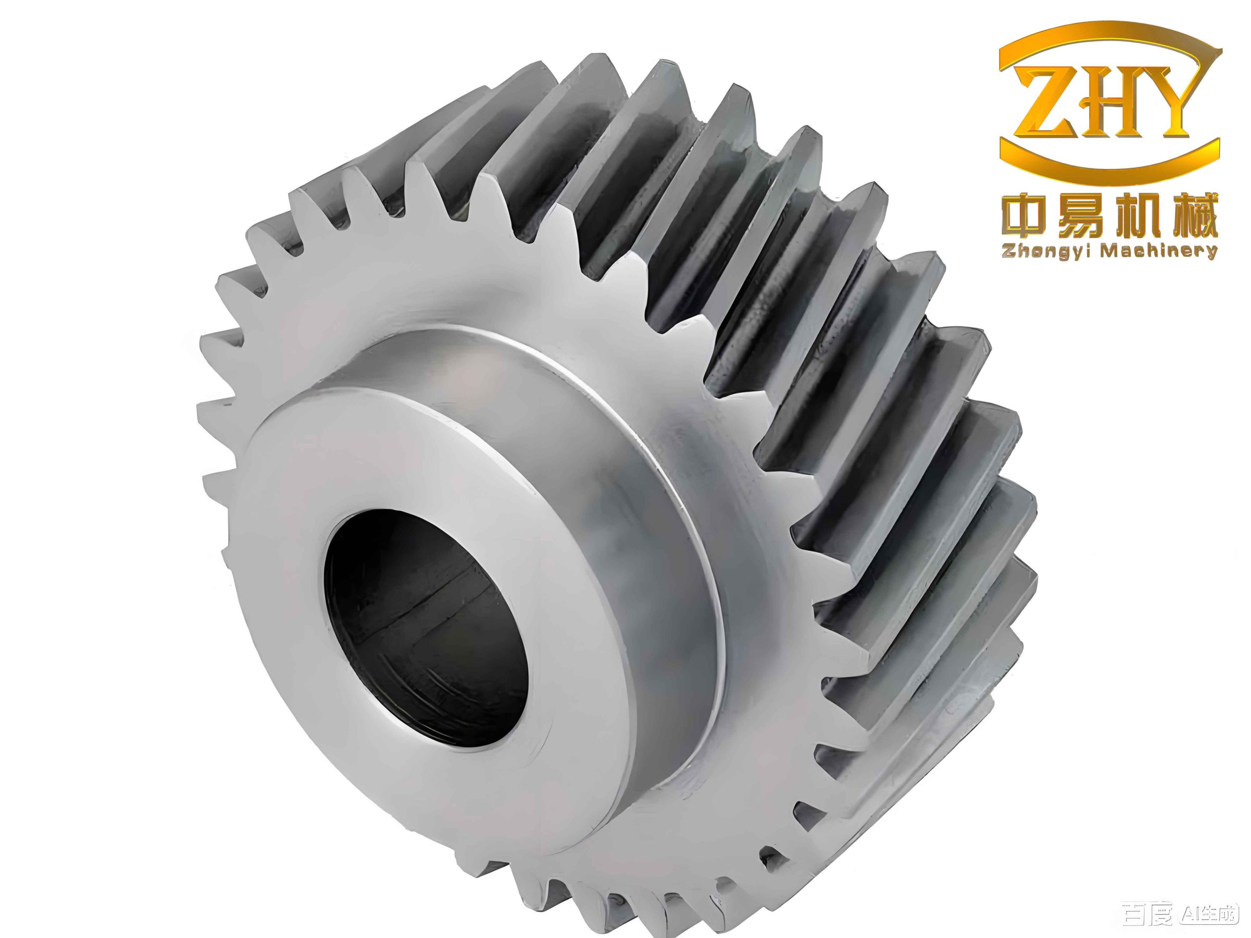
I begin from a practical observation. When a helical gear runs at low speed and high torque, the oil-film shear rate can be large, so the friction force and friction moment are not small. They can alter the dynamic transmission error, the lateral vibration, and the load sharing among contacting tooth pairs. When the same helical gear runs at high speed, the film thickness usually increases, the friction coefficient decreases, and the direct friction effect on the dynamic load becomes weaker. However, the dynamic load itself may still be large because of resonance and coupling among lateral, axial, and torsional motions. Therefore, I treat speed and torque as primary control parameters throughout my analysis.
My modeling framework has three layers. The first layer is the excitation layer, where I compute time-varying mesh stiffness, static transmission error, friction coefficient, friction force, and friction moment. The second layer is the dynamic layer, where I solve single-degree-of-freedom and multi-degree-of-freedom helical gear vibration equations. The third layer is the lubrication layer, where I solve the thermal elastohydrodynamic lubrication equations for finite line contact. I then combine the second and third layers in a unidirectional manner and, finally, in a fully coupled manner. The remainder of this article describes the equations, numerical methods, tables of parameters, and the main trends I obtained.
Parameter excitation for the helical gear mesh. I use an energy-based mesh stiffness model. The total elastic energy of a meshing tooth pair includes Hertz contact energy, bending energy, shear energy, and axial compression energy. The corresponding stiffness components are combined in series to obtain the single-tooth-pair mesh stiffness. For a helical gear, the contact line is inclined relative to the gear axis, and the mesh stiffness varies periodically as the contact line moves across the tooth face. I express the stiffness as a Fourier series because the dynamic solver requires a smooth periodic function. The Hertz contact energy and stiffness are written as
$$U_h=\frac{F^2}{2k_h},\qquad k_h=\frac{\pi E L}{4(1-\nu^2)}.$$
The bending, shear, and axial compression stiffnesses are obtained from cantilever-beam energy expressions. I combine them as
$$\frac{1}{k_m(t)}=\frac{1}{k_h}+\frac{1}{k_{b1}}+\frac{1}{k_{s1}}+\frac{1}{k_{a1}}+\frac{1}{k_{b2}}+\frac{1}{k_{s2}}+\frac{1}{k_{a2}}.$$
For multiple tooth pairs in contact, I superimpose the contributions according to the contact ratio. The static transmission error is represented as a periodic displacement excitation along the line of action,
$$e(t)=e_a\sin(\omega_e t+\phi_e),$$
where $$e_a$$ is the error amplitude, $$\omega_e$$ is the mesh frequency, and $$\phi_e$$ is the phase. I include this term in the dynamic equations because it directly changes the mesh deflection and therefore the dynamic mesh force.
Finite line contact geometry and kinematics. I treat the helical gear contact as two opposite cones in contact. Along the contact line, the curvature radius varies with the contact-line coordinate. I define the coordinate $$y$$ along the contact line and use the base helix angle $$\beta_b$$. The instantaneous radii of curvature of the two helical gear surfaces are
$$r_1(y,t)=r_{d1}(t)-y\sin\beta_b,\qquad r_2(y,t)=r_{d2}(t)+y\sin\beta_b.$$
The equivalent radius and the equivalent curvature are
$$R(y,t)=\frac{R_1R_2}{R_1+R_2},\qquad R_1=r_1\cos\beta_b,\qquad R_2=r_2\cos\beta_b.$$
The surface velocities of the two helical gear flanks are
$$u_1(y,t)=\omega_1(r_{d1}-y\sin\beta_b),\qquad u_2(y,t)=\omega_2(r_{d2}+y\sin\beta_b).$$
The entrainment velocity, sliding velocity, and slide-to-roll ratio are
$$u_e=\frac{u_1+u_2}{2},\qquad u_s=u_1-u_2,\qquad \zeta=\frac{u_s}{u_e}.$$
These kinematic quantities are essential because the friction coefficient of a helical gear depends strongly on entrainment velocity, sliding velocity, contact pressure, and surface roughness. I use a generalized empirical friction coefficient model to estimate the local friction coefficient along the contact line before the fully coupled lubrication calculation is activated. The local friction force and friction moment on a single tooth pair are obtained by integrating the local shear traction over the contact area.
I summarize the primary helical gear parameters used in my study in the following table.
| Parameter | Value | Parameter | Value |
|---|---|---|---|
| Number of teeth, $$z_1,z_2$$ | 28 / 56 | Normal module, $$m_n$$ | 7 mm |
| Pressure angle, $$\alpha$$ | 20 deg | Helix angle, $$\beta$$ | 14 deg |
| Addendum coefficient, $$h_a$$ | 1.0 | Clearance coefficient, $$c$$ | 0.25 |
| Face width, $$B$$ | 15 mm | Elastic modulus, $$E$$ | 227 GPa |
| Input torque, $$T_{in}$$ | 500 N m | Input speed, $$n$$ | 1500 rpm |
Single-degree-of-freedom torsional helical gear model. I first establish a torsional vibration model because it isolates the mesh behavior. The two helical gear bodies are connected by a time-varying mesh stiffness and a mesh damping. The equations are
$$I_1\ddot{\theta}_1+c_m(r_{b1}\dot{\theta}_1-r_{b2}\dot{\theta}_2-\dot e(t))r_{b1}+k(t)(r_{b1}\theta_1-r_{b2}\theta_2-e(t))r_{b1}=T_p+M_1,$$
$$I_2\ddot{\theta}_2-c_m(r_{b1}\dot{\theta}_1-r_{b2}\dot{\theta}_2-\dot e(t))r_{b2}-k(t)(r_{b1}\theta_1-r_{b2}\theta_2-e(t))r_{b2}=-T_g+M_2.$$
I define the relative displacement along the line of action as
$$x=r_{b1}\theta_1-r_{b2}\theta_2-e(t).$$
After introducing the equivalent mass $$m_e=m_1m_2/(m_1+m_2)$$ and the mesh damping $$c_m=2\zeta\sqrt{k_{avg}m_e}$$, the single-degree-of-freedom equation becomes
$$m_e\ddot{x}+c_m\dot{x}+k(t)x=F_s+\frac{m_1+m_2}{m_1m_2}\left(\frac{M_1}{r_{b1}}+\frac{M_2}{r_{b2}}\right)-m_e\ddot e(t).$$
The dynamic mesh force is
$$F_d(t)=c_m\dot{x}+k(t)x.$$
I solve this equation with a variable-order Runge-Kutta method. To improve numerical stability, I nondimensionalize displacement by the Hertzian half-width $$b_H$$, time by the natural period, and force by the average stiffness and half-width. The dimensionless equation is
$$\ddot X+2\zeta \dot X+\bar k(\tau)X=\bar F_s+\bar e(\tau)+\bar M_1+\bar M_2.$$
My single-degree-of-freedom results show that friction has an edge effect on the torsional response. The overall trend of the dynamic transmission error is unchanged, but the curve shifts when friction is included. The shift becomes more visible when the friction coefficient is larger. The dynamic mesh force fluctuates around the static mesh force, and the fluctuation amplitude increases as the speed approaches a resonance. I also find that the critical speed region produces the largest negative dynamic force, which is important for helical gear durability because a negative force indicates a tendency for tooth separation or impact.
The following table summarizes the main dynamic response quantities I extracted from the single-degree-of-freedom model.
| Quantity | Behavior with increasing speed | Effect of friction |
|---|---|---|
| Dynamic transmission error | Amplitude increases, then decreases after resonance | Small shift; edge effect |
| Vibration velocity | Peak near critical speed | Slight change in waveform |
| Vibration acceleration | Strong peak near critical speed | Slight change in waveform |
| Dynamic mesh force | Large fluctuation around static load | Noticeable at high friction coefficient |
Multi-degree-of-freedom helical gear model. A real helical gear system is not purely torsional. Lateral, axial, and torsional motions are coupled through the helix angle and through the bearing supports. I therefore establish an eight-degree-of-freedom model with coordinates
$$[X]^T=[y_1,y_2,x_1,x_2,z_1,z_2,\theta_1,\theta_2]^T.$$
The equations of motion can be written in matrix form as
$$[M]\ddot{[X]}+[C]\dot{[X]}+[K][X]=[P].$$
In expanded form, the lateral, axial, and torsional equations are
$$m_1\ddot y_1+k_{y1}y_1+c_{y1}\dot y_1=-F_d\cos\beta,$$
$$m_2\ddot y_2+k_{y2}y_2+c_{y2}\dot y_2=F_d\cos\beta,$$
$$m_1\ddot x_1+k_{x1}x_1+c_{x1}\dot x_1=f,$$
$$m_2\ddot x_2+k_{x2}x_2+c_{x2}\dot x_2=-f,$$
$$m_1\ddot z_1+k_{z1}z_1+c_{z1}\dot z_1=-F_d\sin\beta,$$
$$m_2\ddot z_2+k_{z2}z_2+c_{z2}\dot z_2=F_d\sin\beta,$$
$$I_1\ddot\theta_1=T_p-F_d r_{b1}\cos\beta-M_1,$$
$$I_2\ddot\theta_2=-T_g+F_d r_{b2}\cos\beta-M_2.$$
The mesh deflection along the normal direction is
$$\delta=(y_1-y_2)\cos\beta+(r_{b1}\theta_1-r_{b2}\theta_2)+(z_1-z_2)\sin\beta-e(t).$$
The dynamic mesh force is
$$F_d=k(t)\delta+c_m\dot\delta.$$
The bearing support forces are computed from the bearing stiffnesses and damping coefficients as
$$F_{byi}=k_{yi}y_i+c_{yi}\dot y_i,\qquad F_{bxi}=k_{xi}x_i+c_{xi}\dot x_i,\qquad F_{bzi}=k_{zi}z_i+c_{zi}\dot z_i.$$
To estimate the natural frequencies, I replace the time-varying mesh stiffness with the average mesh stiffness and solve the symmetric eigenvalue problem. The natural frequencies and corresponding critical speeds are listed below.
| Mode | Eigenvalue | Natural frequency, rad/s | Natural frequency, Hz | Critical speed, rpm |
|---|---|---|---|---|
| y-direction mode 1 | $$2.877\times10^8$$ | $$1.6964\times10^4$$ | $$2.6999\times10^3$$ | $$5.7854\times10^3$$ |
| y-direction mode 2 | $$1.3041\times10^8$$ | $$1.1420\times10^4$$ | $$1.8175\times10^3$$ | $$3.8947\times10^3$$ |
| x-direction mode 1 | $$7.0411\times10^7$$ | $$8.3911\times10^3$$ | $$1.3355\times10^3$$ | $$2.8620\times10^3$$ |
| x-direction mode 2 | $$1.7248\times10^7$$ | $$4.1527\times10^3$$ | $$6.6092\times10^2$$ | $$1.4160\times10^3$$ |
| z-direction mode 1 | $$1.0495\times10^7$$ | $$3.2396\times10^3$$ | $$5.1560\times10^2$$ | $$1.1050\times10^3$$ |
| z-direction mode 2 | $$1.5900\times10^8$$ | $$1.2610\times10^4$$ | $$2.0069\times10^3$$ | $$4.3004\times10^3$$ |
| Torsional coupling mode | $$1.3250\times10^7$$ | $$3.6401\times10^3$$ | $$5.7933\times10^2$$ | $$1.2414\times10^3$$ |
My multi-degree-of-freedom results show that friction has a strong effect on the lateral direction perpendicular to the line of action. This is expected because the friction force acts along that direction. The lateral vibration then changes the surface velocity, which in turn changes the lubrication condition. In contrast, the effect of friction on the torsional motion is weaker for the helical gear parameters I studied. I also observe that the multi-degree-of-freedom model has several resonance peaks, whereas the single-degree-of-freedom model has only one dominant critical speed. At low speed, the dynamic load contains high-frequency components because the mesh stiffness and friction variations are sampled slowly by the tooth engagement. At higher speed, those high-frequency components are filtered by the system inertia and damping.
I compared the single-degree-of-freedom and multi-degree-of-freedom responses at different speeds. At a very high speed, the amplitude difference between the two models is modest. Near a critical speed, the single-degree-of-freedom model can overestimate the dynamic mesh force because it ignores lateral and axial compliance. In the multi-degree-of-freedom model, the resonance peaks are distributed over several speed ranges. This is one reason I use the multi-degree-of-freedom model for the coupled lubrication calculation: it provides a more realistic time history of the dynamic load and surface velocity.
Dynamic response testing. I designed a vibration test to check the qualitative trend of my dynamic model. I mounted a piezoelectric accelerometer on a bearing housing and measured axial acceleration under stable operating conditions. I used a portable acoustic and vibration analyzer to record time-domain and frequency-domain signals. The measured dominant frequency bands were close to the predicted frequency bands from my multi-degree-of-freedom model. The remaining differences came from motor harmonics, support flexibility, and misalignment in the test bench. Because the comparison was qualitative, I used the test only to confirm that the model captures the correct order of magnitude and the main frequency content.
Unidirectional coupling between dynamic load and thermal elastohydrodynamic lubrication. After obtaining the dynamic load from the helical gear dynamic model, I insert it into the lubrication model as the load boundary condition. I solve the finite-line-contact thermal elastohydrodynamic lubrication problem. The Reynolds equation for the lubricant film is
$$\frac{\partial}{\partial x}\left(\frac{\rho h^3}{\eta}\frac{\partial p}{\partial x}\right)+\frac{\partial}{\partial y}\left(\frac{\rho h^3}{\eta}\frac{\partial p}{\partial y}\right)=12u_e\frac{\partial(\rho h)}{\partial x}+12\frac{\partial(\rho h)}{\partial t}.$$
The film thickness equation is
$$h(x,y,t)=h_0(t)+h_g(x,y)+\frac{2}{\pi E’}\iint_\Omega \frac{p(x’,y’,t)}{\sqrt{(x-x’)^2+(y-y’)^2}}dx’dy’+s_1(x,y,t)+s_2(x,y,t).$$
The load balance equation is
$$\iint_\Omega p(x,y,t)dxdy=F_d(t).$$
I use a non-Newtonian lubricant model. The effective viscosity depends on pressure, temperature, and shear stress. The density depends on pressure and temperature. The energy equation for the lubricant film includes convection, conduction, and viscous dissipation. The solid energy equations for the two helical gear flanks include heat conduction and moving heat source effects. The interfacial temperature continuity condition is imposed at the film-solid boundaries. The shear stress on each surface is computed from the pressure gradient, the local viscosity, and the sliding velocity. The friction coefficient is obtained by integrating the shear stress over the contact area and dividing by the normal load.
The lubricant and material properties I used are summarized below.
| Property | Value | Property | Value |
|---|---|---|---|
| Ambient viscosity, $$\eta_0$$ | 0.008 Pa s | Ambient density, $$\rho_0$$ | 870 kg/m$$^3$$ |
| Lubricant specific heat | 2000 J/(kg K) | Solid specific heat | 470 J/(kg K) |
| Lubricant conductivity | 0.14 W/(m K) | Solid conductivity | 46 W/(m K) |
| Pressure-viscosity coefficient | $$2.2\times10^{-8}$$ Pa$$^{-1}$$ | Temperature-viscosity coefficient | 0.0476 K$$^{-1}$$ |
| Ambient temperature | 313 K | Characteristic shear stress | 5 MPa |
I solve the lubrication equations on a finite line contact grid. The pressure field is obtained with a multilevel iteration, and the elastic deformation is computed with a discrete Fourier transform method. The temperature field is solved column by column. I use 128 nodes in the rolling direction, 256 nodes in the contact-line direction, and several nodes across the film thickness. The convergence tolerances are set to very small values for pressure, load, and temperature.
My unidirectional coupling results reveal several important trends for the helical gear. First, the dynamic load is not constant during a mesh cycle. It fluctuates around the static load. As a result, the oil-film pressure and film thickness fluctuate along the line of action. When the dynamic load is larger than the static load, the pressure increases and the film becomes thinner. When the dynamic load is smaller than the static load, the pressure decreases and the film becomes thicker. Second, the temperature field is controlled by both the dynamic load and the sliding velocity. Near the beginning and end of mesh, the sliding velocity is high, so viscous heating is strong. Near the pitch point, the sliding velocity is close to zero, so the temperature rise is small. Third, speed and torque have opposite influences. Increasing speed increases the entrainment velocity and thus increases the film thickness, but it also reduces the friction coefficient. Increasing torque increases the dynamic load, the pressure, and the temperature while reducing the film thickness.
I also studied the effect of tooth surface roughness. When a sinusoidal roughness is superimposed on the smooth surface, the pressure, film thickness, and temperature fields become highly nonuniform. Pressure peaks appear at roughness crests, and pressure valleys appear at roughness troughs. The subsurface stress field shows stress concentration beneath the pressure peaks. This is important for helical gear fatigue because the stress concentration can initiate microcracks even when the average film thickness is acceptable.
The following table summarizes the unidirectional coupling results.
| Factor | Pressure | Film thickness | Temperature | Friction coefficient |
|---|---|---|---|---|
| Increasing speed | Fluctuation becomes stronger | Average film thickness increases | Decreases at high sliding speed | Decreases |
| Increasing torque | Increases | Decreases | Increases | Increases |
| Roughness crest | Local peak | Local minimum | Local hot spot | Local increase |
| Roughness trough | Local valley | Local maximum | Local lower value | Local decrease |
| Pitch point | Moderate | Moderate | Near ambient | Near zero |
Fully coupled tribo-dynamic model for the helical gear. The unidirectional model treats the dynamic load as an input to lubrication. However, the lubrication model produces shear stresses that generate friction forces and friction moments. Those friction quantities act back on the helical gear dynamics. I therefore build a fully coupled model. In this model, the friction force and friction moment are no longer computed from an empirical formula. Instead, they are computed directly from the lubricant shear stress obtained from the thermal elastohydrodynamic lubrication solution.
The friction force on a discrete contact-line station is
$$f_{tj}=\int_{-b_H}^{b_H}\int_{y_j}^{y_{j+1}}\tau(x,y,t)\,dy\,dx.$$
The friction moment on the driving helical gear is
$$M_1=\sum_j f_{tj}r_{1j}+M_{1a}+M_{1b},$$
and the friction moment on the driven helical gear is
$$M_2=\sum_j f_{tj}r_{2j}+M_{2a}+M_{2b}.$$
The surface velocities used in the lubrication calculation include the dynamic motion of the helical gear. I write the instantaneous surface velocities as
$$u_1(y,t)=u_{1a}(y)+r_1(y)\dot\theta_1-\dot x_1,$$
$$u_2(y,t)=u_{2a}(y)+r_2(y)\dot\theta_2-\dot x_2.$$
The terms involving $$\dot x_1$$ and $$\dot x_2$$ represent the lateral vibration contribution. The terms involving $$\dot\theta_1$$ and $$\dot\theta_2$$ represent the torsional vibration contribution. Because these terms are time-dependent, the entrainment velocity and sliding velocity fluctuate even within a single tooth engagement. This fluctuation changes the shear stress, the friction force, and the temperature field.
The coupling iteration proceeds as follows. I first set the friction force and friction moment to zero. I solve the helical gear dynamic equations to obtain the dynamic mesh force and the surface velocities. I then solve the thermal elastohydrodynamic lubrication model to obtain the pressure, film thickness, temperature, and shear stress. I integrate the shear stress to obtain the friction force and friction moment. I substitute those quantities back into the dynamic equations and repeat the process. The iteration stops when the relative change in the dynamic load between two consecutive cycles satisfies
$$\frac{\sum_\gamma |F_d^{(k+1)}(\gamma)-F_d^{(k)}(\gamma)|}{\sum_\gamma |F_d^{(k)}(\gamma)|}<10^{-5}.$$
I summarize the main results of the fully coupled helical gear model below. First, the friction force and friction moment decrease as the rotational speed increases. This happens because the film thickness increases and the effective viscosity in the contact decreases. At low speed, the film is thinner, the shear rate is higher, and the friction force is larger. Second, the effect of friction on the dynamic load is strongest at low speed. When I compare the dynamic load computed with friction and without friction, the difference is small at high speed but noticeable at low speed. Third, the torque level changes the friction force and friction moment, but the relative effect on the dynamic load is less dramatic than the speed effect.
When I examine the pressure and film thickness along the line of action, I find that the coupled model predicts high-frequency fluctuations at low speed. These fluctuations come from the dynamic load and from the lateral vibration contribution to the surface velocity. At higher speed, the high-frequency fluctuations are attenuated, and the pressure and film thickness become smoother. Compared with a static-load lubrication model, the coupled model predicts a different pressure and film-thickness history because the load is redistributed by the dynamics.
The temperature field in the fully coupled model is more realistic than in the static model. The temperature depends on the local sliding speed, the local pressure, and the film thickness. In the coupled model, the lateral vibration changes the sliding speed, so the temperature at a given contact-line position can differ from the static prediction. Near the pitch point, the temperature remains low because the sliding speed is small. Near the beginning and end of mesh, the temperature is higher because the sliding speed is large. The friction torque also changes the torsional velocity, which slightly modifies the entrainment velocity and therefore the film thickness.
The friction coefficient in the fully coupled model is generally lower than in the static model. This is because the dynamic lateral motion modifies the entrainment and sliding velocities in a way that reduces the effective shear stress. The reduction is more pronounced at low speed, where the friction coefficient is already high and the friction force has a stronger influence on the dynamic response.
The following table compares the static lubrication model and the fully coupled tribo-dynamic model for the helical gear.
| Feature | Static lubrication model | Fully coupled tribo-dynamic model |
|---|---|---|
| Load input | Constant nominal load | Time-varying dynamic load |
| Surface velocity | Kinematic average velocity | Average velocity plus lateral and torsional vibration |
| Pressure history | Smooth along line of action | Fluctuating, especially at low speed |
| Film thickness | Smooth | High-frequency fluctuation at low speed |
| Temperature | Mainly sliding-speed controlled | Sliding-speed and dynamic-load controlled |
| Friction coefficient | Higher at low speed | Lower because of dynamic velocity modulation |
| Fatigue indicator | Steady subsurface stress | Stress concentration under dynamic pressure peaks |
Discussion of speed and torque effects. Speed and torque are the two external variables I examined most carefully. At very low speed, the helical gear operates close to a mixed or boundary lubrication condition if the roughness is significant. The oil-film shear stress is high, and the friction force is large. The dynamic load is close to the static load in magnitude, but it contains high-frequency oscillations. These oscillations can cause repeated local pressure spikes and temperature spikes. At intermediate speed, the film thickness increases, and the friction coefficient decreases. The dynamic load begins to show resonant amplification. At high speed, the film thickness is large, and the friction coefficient is small. The direct friction effect on the dynamic load is weak, but the dynamic load may still be large because of resonance and because of the coupling among lateral, axial, and torsional motions.
Torque mainly changes the mean load. As torque increases, the static mesh force increases, the dynamic mesh force increases, the oil-film pressure increases, and the film thickness decreases. The friction coefficient also increases because the pressure increases and the film becomes thinner. The temperature increases because the viscous dissipation and the sliding heat generation increase. The dynamic transmission error increases with torque because the elastic deformation of the teeth and the contact becomes larger.
The following table lists the observed trends in the fully coupled helical gear model.
| Condition | Dynamic load | Friction force | Film thickness | Temperature |
|---|---|---|---|---|
| Low speed, low torque | Close to static, high-frequency ripple | Moderate | Thin | Moderate |
| Low speed, high torque | High mean, high-frequency ripple | High | Very thin | High |
| Medium speed, medium torque | Resonance possible | Moderate | Moderate | Moderate |
| High speed, low torque | Dynamic amplification possible | Low | Thick | Low to moderate |
| High speed, high torque | High mean and dynamic load | Moderate | Moderate | High |
Numerical implementation and convergence. I implemented the dynamic solver and the lubrication solver in a coupled loop. The dynamic equations are solved with a variable-order Runge-Kutta method. The lubrication equations are solved with a multilevel pressure iteration, a discrete Fourier transform for elastic deformation, and a column-sweep method for temperature. The contact grid is sufficiently fine to resolve the finite line contact and the roughness-induced pressure fluctuations. I use a dimensionless formulation for both the dynamic and lubrication variables. The dimensionless groups include the speed parameter, the load parameter, the material parameter, and the thermal parameter. This makes the numerical results more general and improves convergence.
The coupled iteration is stable when the relaxation factor is chosen carefully. I use under-relaxation for the friction force and friction moment in the first few iterations, and then I switch to direct substitution when the residual is small. The convergence criterion is based on the relative change in the dynamic load over one mesh cycle. I also monitor the pressure residual and the temperature residual to ensure that the lubrication solution is converged at each coupling step.
Implications for helical gear design and fatigue. My results show that the traditional practice of using a constant load in helical gear lubrication analysis can miss important transient effects. The dynamic load changes the pressure and film thickness along the line of action. The friction force and friction moment change the lateral and torsional vibration. The lateral vibration changes the surface velocity and therefore the lubricant shear stress. This closed loop means that the lubrication condition and the dynamic condition must be evaluated together. For fatigue life prediction, the subsurface stress field should be computed from the coupled pressure distribution rather than from a static pressure distribution. The roughness-induced pressure peaks are particularly important because they create local stress concentrations that can initiate pitting or micropitting.
For a helical gear designer, the practical implications are as follows. First, if the helical gear operates at low speed and high torque, friction should not be neglected in the dynamic model. Second, if the helical gear operates near a system resonance, the dynamic load should be used as the lubrication input even if the friction coefficient is small. Third, if the tooth surface is rough, the lubrication analysis should include roughness because the pressure peaks and subsurface stress concentrations can dominate the fatigue behavior. Fourth, if the helical gear is lightly loaded, the friction effect on the dynamic load is small, but the dynamic load may still be amplified by resonance. Fifth, the axial and lateral support stiffnesses should be included because they change the natural frequencies and the mode shapes of the helical gear system.
Summary of my main findings. I established a finite-line-contact tribo-dynamic framework for a helical gear pair. I derived the time-varying mesh stiffness, the static transmission error, the contact kinematics, the friction force, and the friction moment. I solved the single-degree-of-freedom and multi-degree-of-freedom dynamic equations. I solved the thermal elastohydrodynamic lubrication equations for finite line contact. I coupled the dynamic and lubrication models in a unidirectional manner and then in a fully coupled manner. The main findings are the following.
First, the dynamic mesh force of a helical gear fluctuates around the static mesh force. The fluctuation amplitude depends on speed and on the proximity to a natural frequency. The multi-degree-of-freedom model predicts several resonance regions, whereas the single-degree-of-freedom model predicts one dominant critical speed.
Second, friction has a weak effect on the torsional motion of the helical gear but a strong effect on the lateral motion perpendicular to the line of action. Because the lateral motion changes the surface velocity, friction indirectly changes the lubrication condition. This indirect effect is important for the fully coupled response.
Third, the dynamic load changes the oil-film pressure and film thickness along the line of action. When the dynamic load is larger than the static load, the pressure is higher and the film is thinner. When the dynamic load is smaller than the static load, the pressure is lower and the film is thicker. At low speed, the pressure and film thickness can contain high-frequency fluctuations. At high speed, those fluctuations are reduced.
Fourth, the temperature field is controlled by the sliding speed and the dynamic load. Near the pitch point, the sliding speed is small, so the temperature rise is small. Near the beginning and end of mesh, the sliding speed is large, so the temperature rise is large. The dynamic load increases the local pressure and therefore increases the local temperature.
Fifth, roughness creates local pressure peaks and subsurface stress concentrations. The pressure peaks are located at roughness crests, and the pressure valleys are located at roughness troughs. The subsurface stress concentration follows the pressure peaks. This is a key mechanism for surface-initiated fatigue in a helical gear.
Sixth, the fully coupled model predicts a lower friction coefficient than the static model because the lateral and torsional vibrations modify the entrainment and sliding velocities. The effect is strongest at low speed, where the friction force is large. At high speed, the friction coefficient is small, and the difference between the coupled and static models is less pronounced.
Final remarks. I conclude that a helical gear should be analyzed as a coupled tribo-dynamic system when the operating speed and torque are variable and when the tooth load is time-dependent. The finite line contact formulation is necessary because the contact line length changes during mesh, and the end rounding of the helical gear tooth affects the pressure distribution. The thermal elastohydrodynamic lubrication model is necessary because the lubricant viscosity and film thickness depend strongly on temperature. The dynamic model is necessary because the mesh stiffness, transmission error, and friction excitation cause time-varying loads and vibrations. The fully coupled model combines these effects and provides a more realistic prediction of pressure, film thickness, temperature, friction coefficient, and subsurface stress. I plan to extend this framework to helical gears with surface defects, pitting, and cracks, and to use the coupled pressure and stress fields to estimate fatigue initiation life under realistic operating conditions.