
In this study, I focus on the dynamic behavior of helical gears used in high-speed train gearboxes. Helical gears are widely applied because they offer high transmission efficiency, smooth operation, and strong load-carrying capacity. However, long-term service under high speed and heavy load makes helical gears susceptible to root cracks and surface spalling. These faults reduce mesh stiffness and intensify vibration, which threatens the stability and safety of train operation. My goal is to establish a relationship between fault parameters and dynamic features so that condition monitoring and fault diagnosis of helical gears can be improved. I build a nonlinear dynamic model of a helical gear system, calculate time-varying mesh stiffness with fault effects, and solve the dynamic response under different fault conditions. The results show that crack and spalling faults significantly alter the periodic motion, bifurcation behavior, and frequency content of helical gears.
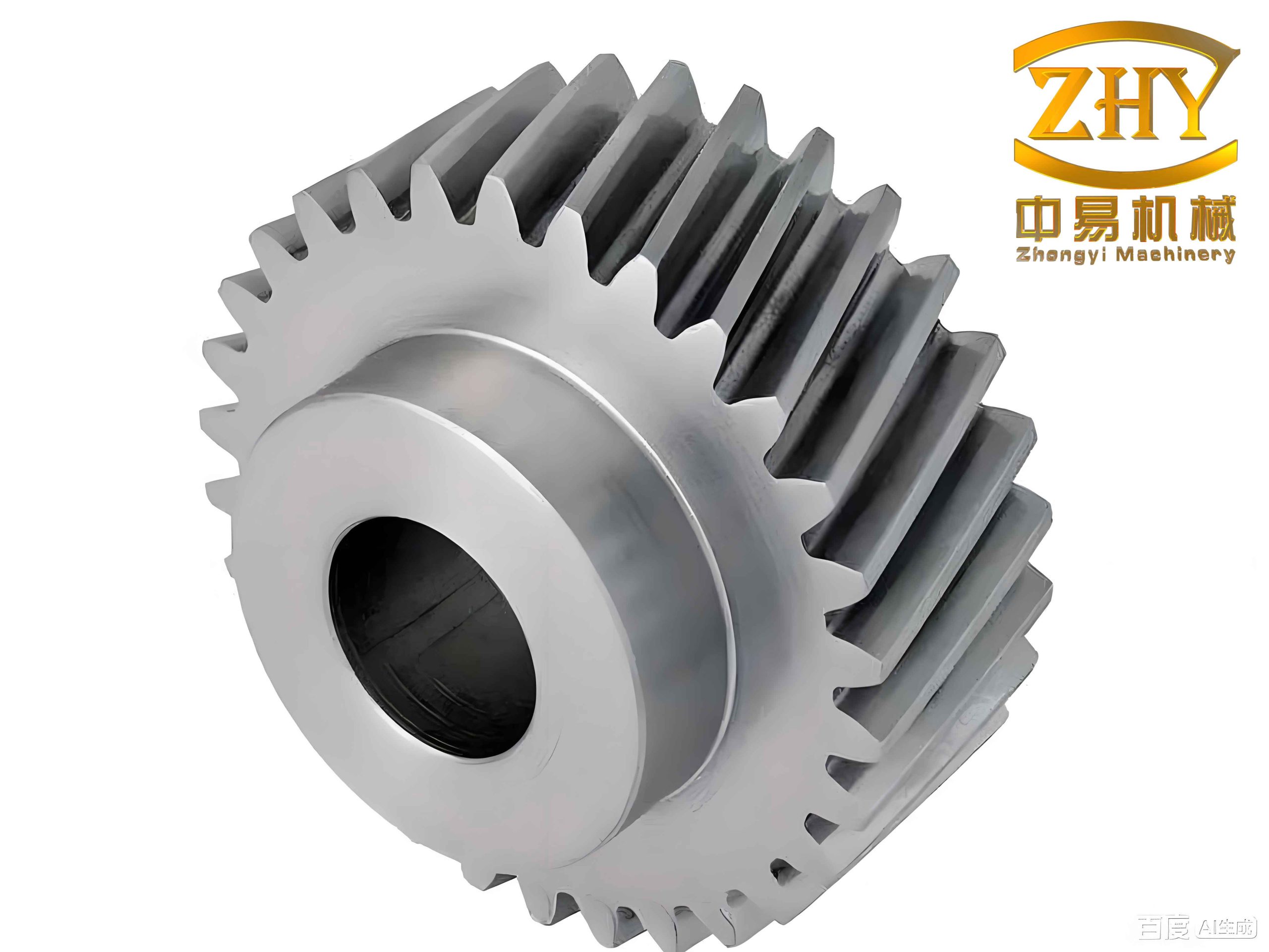
I consider four main nonlinear factors in the helical gear system: time-varying mesh stiffness, backlash, mesh damping, and transmission error. These factors are internal excitations that distinguish gear systems from other mechanical systems. Time-varying mesh stiffness is caused by the periodic change in the number of contacting tooth pairs and the variation of contact position along the tooth profile. Backlash exists for assembly, lubrication, and thermal expansion, but excessive backlash can cause impact and noise. Mesh damping dissipates vibration energy through friction and deformation. Transmission error represents the difference between the theoretical and actual positions along the line of action. To model the helical gear system, I use the lumped mass method and Newton’s second law. The model has six degrees of freedom: translations in the y and z directions and rotations about the gear axes for both pinion and gear. I assume that tooth friction is neglected, shaft mass is concentrated on the gears, and the gear bodies are rigid. The interaction between helical gears is represented by a stiffness-damping element.
The dynamic equations of the helical gear system can be written as follows:
$$
\begin{aligned}
I_1 \ddot{\theta}_1 + r_{b1} F_d &= T_1, \\
I_2 \ddot{\theta}_2 – r_{b2} F_d &= -T_2, \\
m_1 \ddot{y}_1 + c_{1y} \dot{y}_1 + k_{1y} y_1 &= F_y, \\
m_2 \ddot{y}_2 + c_{2y} \dot{y}_2 + k_{2y} y_2 &= -F_y, \\
m_1 \ddot{z}_1 + c_{1z} \dot{z}_1 + k_{1z} z_1 &= F_z, \\
m_2 \ddot{z}_2 + c_{2z} \dot{z}_2 + k_{2z} z_2 &= -F_z.
\end{aligned}
$$
Here, \(F_d\) is the dynamic mesh force, \(F_y\) and \(F_z\) are its components along the y and z directions. The dynamic mesh force is expressed as:
$$
F_d = k(t) \delta(t) + c_m \dot{\delta}(t),
$$
$$
F_y = F_d \cos \beta_b, \quad F_z = F_d \sin \beta_b,
$$
where \(k(t)\) is the time-varying mesh stiffness, \(c_m\) is the mesh damping, and \(\beta_b\) is the base helix angle. The dynamic transmission error \(\delta(t)\) is given by:
$$
\delta(t) = y_1 – y_2 – z_1 \sin \beta_b – z_2 \sin \beta_b + r_{b1} \theta_1 – r_{b2} \theta_2 – e(t) \cos \beta_b.
$$
The backlash function \(f(\delta)\) is defined as:
$$
f(\delta) =
\begin{cases}
\delta – b, & \delta > b, \\
0, & -b \leq \delta \leq b, \\
\delta + b, & \delta < -b,
\end{cases}
$$
where \(b\) is half of the backlash. The mesh damping is calculated by an empirical formula:
$$
c_m = 2 \xi_g \sqrt{\frac{k_m r_{b1}^2 r_{b2}^2 I_1 I_2}{r_{b1}^2 I_1 + r_{b2}^2 I_2}},
$$
where \(\xi_g\) is the damping ratio and \(k_m\) is the average mesh stiffness. The transmission error is represented by a Fourier series, and only the first harmonic is retained:
$$
e(t) = e_0 + e_1 \cos(\omega_m t + \varphi_1),
$$
where \(\omega_m\) is the mesh frequency. I introduce a dimensionless time scale \(\tau = \omega_n t\) with \(\omega_n = \sqrt{k_m / m_e}\), and dimensionless displacement \(Y_i = y_i / b\), \(Z_i = z_i / b\), \(\lambda = \delta(t) / b\). The state equations are then derived by reducing the second-order equations to first-order form. The dimensionless parameters are listed in Table 1.
| Parameter | Symbol | Pinion | Gear |
|---|---|---|---|
| Number of teeth | \(z\) | 29 | 69 |
| Normal module (mm) | \(m_n\) | 7 | 7 |
| Normal pressure angle (deg) | \(\alpha_n\) | 26 | 26 |
| Helix angle (deg) | \(\beta\) | 20 | 20 |
| Face width (mm) | \(B\) | 75 | 70 |
| Addendum coefficient | \(h_{an}^*\) | 1 | 1 |
| Clearance coefficient | \(c_n^*\) | 0.25 | 0.25 |
| Load (N m) | \(T\) | 3500 | 3500 |
| Young’s modulus (Pa) | \(E\) | \(2.06 \times 10^{11}\) | \(2.06 \times 10^{11}\) |
| Poisson’s ratio | \(\nu\) | 0.3 | 0.3 |
| Inner radius (mm) | \(r_{int}\) | 48 | 100 |
For helical gears, the contact line is inclined with respect to the tooth width. I use the slice theory to divide each helical gear tooth into a number of thin slices along the face width. When the slice is sufficiently thin, each slice can be treated as a spur gear tooth. The total mesh stiffness of helical gears at a given meshing position is the sum of the stiffness of all slices:
$$
K = \sum_{i=1}^{M} k_i,
$$
where \(M\) is the number of slices in contact. The number of slices \(N\) along the face width is determined by:
$$
N = \left\lfloor \frac{L_1 N_1}{L_1 \tan \beta_b} \right\rfloor,
$$
where \(L_1 = \varepsilon_\alpha p_{bt}\), \(\varepsilon_\alpha\) is the transverse contact ratio, and \(p_{bt}\) is the transverse base pitch. Each slice has a width \(\Delta y = L_1 / (N_1 \tan \beta_b)\). In my study, the helical gears have a contact ratio of 2.53, so up to three tooth pairs can be in contact simultaneously.
To calculate the mesh stiffness accurately, I model the real tooth profile. The tooth profile consists of three parts: the root transition curve, the involute profile, and the tip arc. The transition curve connects the root circle and the base circle. In many studies, this transition curve is simplified as a straight line or ignored, but this introduces errors. I use the exact equation of the transition curve generated by a rack cutter with a tip radius. The transition curve is given by:
$$
\begin{aligned}
x &= r – \left( a_1 – \frac{r_\rho}{\sin \gamma} \right) \cos \gamma + r_\rho \sin \gamma, \\
y &= r – \left( a_1 – \frac{r_\rho}{\sin \gamma} \right) \sin \gamma – r_\rho \cos \gamma,
\end{aligned}
$$
where \(r\) is the pitch radius, \(a_1\) and \(r_\rho\) are tool parameters, and \(\gamma\) is a parameter. The involute profile is described by:
$$
x = r_i \cos \tau, \quad y = r_i \sin \tau,
$$
with \(r_i = r_b / \cos \alpha_i\), \(\tau = \pi / (2z) + \theta_t – \theta_i\), \(\theta_t = \tan \alpha_t – \alpha_t\), and \(\theta_i = \tan \alpha_i – \alpha_i\). Here, \(r_b\) is the base radius and \(\alpha_t\) is the transverse pressure angle. Using these equations, I generate an accurate tooth profile model for the helical gears.
I apply the potential energy method to calculate the stiffness of each slice. The tooth is treated as a cantilever beam fixed at the root circle. The total potential energy includes bending, shear, axial compression, Hertzian contact, and fillet foundation deformation. The bending stiffness \(k_b\), shear stiffness \(k_s\), and axial compression stiffness \(k_a\) are obtained from:
$$
\frac{1}{k_b} = \int_0^d \frac{[(d-x)\cos \alpha_1 – h \sin \alpha_1]^2}{E I_x} dx,
$$
$$
\frac{1}{k_s} = \int_0^d \frac{1.2 \cos^2 \alpha_1}{G A_x} dx,
$$
$$
\frac{1}{k_a} = \int_0^d \frac{\sin^2 \alpha_1}{E A_x} dx,
$$
where \(d\) is the horizontal distance from the meshing point to the root, \(h\) is the distance from the meshing point to the tooth centerline, \(\alpha_1\) is the meshing angle, \(E\) is Young’s modulus, \(G = E / [2(1+\nu)]\) is the shear modulus, and \(I_x\) and \(A_x\) are the area moment of inertia and cross-sectional area at distance \(x\) from the root. The Hertzian contact stiffness \(k_h\) is:
$$
k_h = \frac{\pi E \Delta y}{4(1-\nu^2) \cos \beta_b}.
$$
The fillet foundation stiffness \(k_f\) is calculated using an analytical formula:
$$
\frac{1}{k_f} = \frac{\cos^2 \alpha_1}{E \Delta y} \left[ L^* \left( \frac{u_f}{S_f} \right)^2 + M^* \left( \frac{u_f}{S_f} \right) + P^* \left( 1 + Q^* \tan^2 \alpha_1 \right) \right],
$$
where \(u_f\) and \(S_f\) are geometric parameters, and \(L^*, M^*, P^*, Q^*\) are polynomial coefficients. For a single tooth pair, the stiffness \(k\) is the series combination:
$$
k = \left( \frac{1}{k_{t1}} + \frac{1}{k_{t2}} + \frac{1}{k_h} + \frac{1}{k_{f1}} + \frac{1}{k_{f2}} \right)^{-1},
$$
where \(k_{ti} = 1/(1/k_{si} + 1/k_{ai} + 1/k_{bi})\). The total mesh stiffness of helical gears with multiple tooth pairs is the parallel sum:
$$
K_z = \sum_{i=1}^{n} K_i.
$$
To account for the axial force effect, I apply a correction factor:
$$
K = k \cos^2 \beta_b.
$$
I verify the analytical model using the finite element method. I build a three-dimensional model of five tooth pairs and perform transient dynamic analysis. I apply a torque of 3500 N m to the driven gear and extract the rotation angles. The mesh stiffness from finite element analysis is calculated by:
$$
k = \frac{T_2}{r_{b1}^2 [\theta_1(t) – \theta_2(t)] r_{b2} – r_{b1} e(t)}.
$$
The comparison shows that the average error between my analytical method and the finite element method is 2.58%, and the maximum error is 4.52%. This confirms that my model can accurately calculate the time-varying mesh stiffness of helical gears. The slight underestimation is due to neglecting shear stress between slices. For dynamic simulations, I need a continuous stiffness function. I compare linear interpolation and Fourier series fitting. The linear interpolation method gives an almost zero relative error, while the Fourier series method has a maximum error of 1.21%, especially near stiffness jumps. Therefore, I use linear interpolation for the mesh stiffness of helical gears.
To study crack faults, I establish a non-uniform root crack model. In reality, a crack does not propagate uniformly along the tooth width in its early stages. I assume that the crack depth follows a parabolic distribution along the face width for a through crack, and a linear distribution for a non-through crack. The crack depth \(q(z)\) at position \(z\) is:
$$
q(z) = q_0 + \frac{2(q_e – q_0)}{L^2} z^2,
$$
for a through crack, and
$$
\begin{cases}
q(z) = q_0 – \frac{q_0}{L_c} z, & 0 \leq z \leq L_c, \\
q(z) = 0, & L_c < z \leq L,
\end{cases}
$$
for a non-through crack. Here, \(q_0\) is the crack depth at the front face, \(q_e\) is the depth at the back face, \(L\) is the face width, and \(L_c\) is the crack length. I define the crack percentage as the ratio of the cracked area to the total cross-sectional area. Five crack cases are summarized in Table 2.
| Case | \(q_0\) (mm) | \(q_e\) (mm) | \(L_c\) (mm) | Crack percentage |
|---|---|---|---|---|
| Case 1 | 0 | 0 | 0 | 0 |
| Case 2 | 4 | 0 | 45 | 13% |
| Case 3 | 6 | 0 | 60 | 27% |
| Case 4 | 8 | 0 | 75 | 44% |
| Case 5 | 10 | 3 | 75 | 60% |
| Case 6 | 12 | 6 | 75 | 78% |
When a crack occurs, the cross-sectional area and area moment of inertia of the cracked tooth slice are reduced. The crack does not affect the axial compression stiffness, contact stiffness, or fillet foundation stiffness, but it changes the bending and shear stiffness. I derive the modified area and inertia for two cases: when the crack does not pass through the base and when it does. The reduced area \(A_{x,crack}\) and inertia \(I_{x,crack}\) are used in the potential energy integrals. Then, the bending and shear stiffness of the cracked slice are obtained. Summing over all slices gives the total bending and shear stiffness of the cracked helical gear. The single tooth pair stiffness with a crack is:
$$
k_{crack} = \left( \frac{1}{k_{s,crack}} + \frac{1}{k_{b,crack}} + \frac{1}{k_a} + \frac{1}{k_f} + \frac{1}{k_h} \right)^{-1}.
$$
I define the stiffness reduction percentage \(P\) as:
$$
P = \frac{k_0 – k_c}{k_0} \times 100\%,
$$
where \(k_0\) is the mesh stiffness of a healthy gear and \(k_c\) is the mesh stiffness of a cracked gear. The results show that as the crack severity increases, the mesh stiffness of helical gears decreases, and the reduction amount increases. For the same crack, the reduction first increases and then decreases, and the maximum reduction occurs in the double-tooth contact zone near the tooth tip. For example, in Case 6, the mesh stiffness decreases by 10.85% at the position where the pinion rotates 0.38 rad. This is because the cracked slices are most numerous at that position, and the double-tooth zone has lower stiffness than the triple-tooth zone. Therefore, for helical gears with root cracks, attention should be paid to the double-tooth contact zone near the tip.
For spalling faults, I use a rectangular spalling model. The spall is defined by length \(l_s\), width \(w_s\), depth \(h_s\), and initial position \(x_{start}\). The spall is symmetric about the tooth width centerline. The spalled tooth slice has a reduced cross-sectional area and inertia. The reduced area is:
$$
dA_x = (h_x – h_s) \Delta y, \quad x_{start} \leq x \leq x_{end}.
$$
The neutral axis shifts by \(\delta_{xs}\), and the reduced inertia is:
$$
dI_x = \frac{(h_x – h_s)^3}{12} \Delta y + (h_x – h_s) \Delta y \, \delta_{xs}^2.
$$
The spall also reduces the effective contact line length. The contact stiffness of a spalled slice becomes zero when the meshing point is inside the spall region. The total stiffness of the spalled helical gear is obtained by summing the healthy slices and the spalled slices. I study the influence of spall parameters on mesh stiffness. The results show that spalling causes a local reduction in mesh stiffness. Among the four parameters, spall length has the largest effect. For a given spall, as the tooth engages, the stiffness reduction first increases sharply, then slowly, then sharply again, and finally remains constant. The spall width and depth do not change the range of the affected zone, but increasing the spall width moves the maximum reduction position toward the tooth tip. Moving the initial spall position toward the tip reduces the affected zone. Increasing the spall length both expands the affected zone and significantly reduces the mesh stiffness.
After calculating the mesh stiffness of healthy, cracked, and spalled helical gears, I solve the dynamic response using the standard fourth-order Runge-Kutta method. The dynamic simulation parameters are listed in Table 3.
| Parameter | Symbol | Pinion | Gear |
|---|---|---|---|
| Mass (kg) | \(m\) | 9.65 | 56.92 |
| Bearing stiffness in y (N/m) | \(k_y\) | \(2.5 \times 10^7\) | \(2.5 \times 10^7\) |
| Bearing stiffness in z (N/m) | \(k_z\) | \(2.5 \times 10^7\) | \(2.5 \times 10^7\) |
| Bearing damping in y (N s/m) | \(c_y\) | \(1 \times 10^4\) | \(1 \times 10^4\) |
| Bearing damping in z (N s/m) | \(c_z\) | \(1 \times 10^4\) | \(1 \times 10^4\) |
| Backlash (μm) | \(b\) | 40 | 40 |
| Transmission error amplitude (μm) | \(e\) | 10 | 10 |
| Damping ratio | \(\xi\) | 0.03 | 0.03 |
For the healthy helical gear system, I analyze the bifurcation behavior as the pinion speed increases from 1000 to 10000 rpm. The system exhibits rich nonlinear behavior. At low speeds from 1000 to 6300 rpm, the system is period-1, except for a jump phenomenon at 4700 rpm. At 3500 rpm, the phase trajectory shows multiple closed curves, the Poincaré section shows a point cluster, and the frequency spectrum is dominated by the mesh frequency \(f_m\) and its harmonics, indicating quasi-periodic motion. At 5000 rpm, the phase trajectory is a single closed curve, the Poincaré section is a point, and the spectrum is dominated by \(f_m\) and its harmonics, indicating period-1 motion. At 6500 rpm, the system becomes period-2, with two closed curves and two points in the Poincaré section. The spectrum shows the half mesh frequency \(f_m/2\). At 7000 rpm, the system becomes chaotic, with entangled curves and a continuous spectrum. At 7500 rpm, the system is period-4. At 8400 rpm, the system is period-5. The healthy system experiences period-1, multi-period, and chaotic motions, showing strong nonlinearity.
When a root crack occurs, the dynamic behavior changes significantly. I use a crack with angle 60°, \(q_0 = 8\) mm, \(q_e = 0\) mm, and \(L_c = 75\) mm. The bifurcation diagram and maximum Lyapunov exponent show that the crack causes the system to change from periodic to quasi-periodic, multi-periodic, or chaotic motion. The bifurcation points become scattered, and the chaotic range increases. At speeds below 6500 rpm, the system changes from period-1 to period-3. At speeds above 6500 rpm, the system changes from periodic to quasi-periodic or chaotic. For example, at 9800 rpm, the maximum Lyapunov exponent changes from negative to positive, indicating chaos. The crack also increases the maximum Lyapunov exponent, which means the system stability decreases. At low speed, such as 3500 rpm, the healthy system is period-1, while the cracked system is period-3. The time-domain signal shows periodic impacts with a period equal to the rotation period of the cracked gear \(T_s = 60/n\). The spectrum shows fault characteristic frequency \(f_s = n/60\) and its harmonics around the mesh frequency. At medium speed, such as 6500 rpm, the cracked system becomes quasi-periodic period-2. The time-domain impact is not obvious because the impact energy is distributed over a wider frequency band. At high speed, such as 9900 rpm, the cracked system becomes chaotic, with a continuous spectrum. The maximum Lyapunov exponent changes from negative to positive, confirming the loss of stability.
I also analyze the dynamic mesh force. The maximum mesh force indicates the tooth surface impact state, and the minimum mesh force indicates the back impact state. For the healthy system, when speed is below 4700 rpm, both maximum and minimum mesh forces are positive, so the system is in a no-impact state. When speed is between 4700 and 10000 rpm, the maximum mesh force is positive and the minimum is negative, so the system is in a double-sided impact state. At 4700 rpm, the system is in a single-sided impact state. The crack fault has little effect on the maximum and minimum mesh forces, except at speeds below 2100 rpm where the crack increases the maximum mesh force.
For crack evolution, I vary the crack percentage from 0 to 78% and analyze the system at different speeds. At 5400 rpm, the bifurcation diagram shows that as the crack severity increases, the vibration amplitude increases. When the crack percentage is below 22%, the amplitude does not change much. When it exceeds 22%, the number of periodic motions increases and the amplitude grows. The three-dimensional phase trajectory, Poincaré section, time-domain, and frequency spectrum show that with crack growth, the phase trajectory diverges, the number of closed curves increases, and the fault characteristic frequency amplitude increases. At 7600 rpm, the healthy system is period-4. As the crack grows, the system transitions to quasi-periodic period-4 and then to chaos. The time-domain signal becomes disordered, and the spectrum shows a continuous component. The fault feature becomes harder to identify at high speed.
For spalling faults, I use a spall with length \(l_s = 35\) mm, depth \(h_s = 1.2\) mm, width \(w_s = 4\) mm, and initial position \(x_{start} = 97.3\) mm. The bifurcation diagram and maximum Lyapunov exponent show that spalling causes the system to change from period-1 to multi-period or quasi-periodic motion. The chaotic range increases, and the speed at which chaos begins is lower. The maximum Lyapunov exponent increases, indicating reduced stability. At low speed, such as 3000 rpm, the healthy system is period-1, while the spalled system is period-2. The time-domain signal shows periodic impacts with a period equal to the rotation period of the spalled gear. The spectrum shows sidebands around the mesh frequency, with the sideband spacing equal to the fault characteristic frequency. At medium speed, such as 7500 rpm, the healthy system is period-4, while the spalled system becomes quasi-periodic period-4. At high speed, such as 9500 rpm, both healthy and spalled systems are chaotic, but the spalling increases the amplitude of the 1/3 mesh frequency. The dynamic mesh force analysis shows that spalling does not change the impact state, but it increases the maximum mesh force at speeds below 2500 rpm.
For spall evolution, I vary the spall length from 0 to 70 mm. At 6500 rpm, the healthy system is period-2. As the spall length increases, the system transitions from period-2 to quasi-periodic period-2 and then to multi-period motion. The three-dimensional phase trajectory diverges, the Poincaré section changes from two points to two point clusters and then to two lines. The time-domain impact sequence becomes more obvious, and the fault characteristic frequency amplitude increases. At 8500 rpm, the healthy system is period-5. As the spall length increases, the system becomes quasi-periodic period-5, then chaotic, and finally chaotic. The time-domain signal becomes disordered, and the spectrum shows a continuous component. When the spall length is too long, the fault feature frequency evolves into a continuous spectrum, making identification difficult.
To evaluate the health condition of helical gears, I use five time-domain statistical indicators: kurtosis, root mean square (RMS), shape factor, crest factor, and impulse factor. Their formulas are:
$$
K = \frac{\frac{1}{N} \sum_{i=1}^N (x_i – \bar{x})^4}{\left[ \frac{1}{N} \sum_{i=1}^N (x_i – \bar{x})^2 \right]^2},
$$
$$
RMS = \sqrt{\frac{1}{N} \sum_{i=1}^N (x_i – \bar{x})^2},
$$
$$
W_f = \frac{RMS}{\frac{1}{N} \sum_{i=1}^N |x_i|},
$$
$$
P_f = \frac{x_p}{RMS},
$$
$$
I_f = \frac{x_p}{\frac{1}{N} \sum_{i=1}^N |x_i|},
$$
where \(x_i\) is the vibration signal, \(x_p\) is the peak value, \(N\) is the number of samples, and \(\bar{x}\) is the mean. I use two methods. Method 1 calculates the indicators of the difference signal between the fault signal and the healthy signal. Method 2 calculates the percentage change of the indicators relative to the healthy condition. The results show that for crack faults, the shape factor and crest factor from Method 1 increase monotonically with crack severity, while other indicators remain nearly constant. For spalling faults, the shape factor and crest factor from Method 1 also increase monotonically with spall length. Method 2 does not show a clear monotonic trend. Therefore, the crest factor and shape factor from Method 1 are effective indicators for evaluating the fault severity of helical gears.
| Indicator | Crack sensitivity | Spalling sensitivity | Trend |
|---|---|---|---|
| Kurtosis | Low | Low | Non-monotonic |
| RMS | Low | Low | Nearly constant |
| Shape factor | High | High | Monotonic increase |
| Crest factor | High | High | Monotonic increase |
| Impulse factor | Low | Low | Nearly constant |
Based on my analysis, I draw several conclusions. First, the analytical mesh stiffness model for helical gears, which considers the exact tooth profile including the transition curve, agrees well with finite element results. The average error is 2.58%, and the maximum error is 4.52%. Linear interpolation is better than Fourier series for fitting the mesh stiffness of helical gears. Second, crack faults reduce the mesh stiffness of helical gears, and the reduction increases with crack severity. The maximum reduction occurs in the double-tooth contact zone near the tooth tip. Spalling causes local stiffness reduction, and spall length has the largest influence among the four parameters. Third, both crack and spalling faults change the dynamic behavior of helical gears. At low speeds, faults change period-1 motion to multi-period motion, and the time-domain signal shows obvious periodic impacts. The spectrum shows fault characteristic frequencies. At high speeds, faults change periodic motion to quasi-periodic or chaotic motion, and the time-domain impacts and fault frequencies become difficult to observe. Therefore, low-speed conditions are more suitable for early fault detection of helical gears. Fourth, as faults evolve, the periodic motion behavior changes, and the change process differs at different speeds. At low speeds, the number of periodic motions increases, and the fault features become more identifiable. At high speeds, the system transitions from periodic to quasi-periodic and then to chaos, with a continuous spectrum. Finally, the crest factor and shape factor calculated from the difference signal are effective indicators for evaluating the fault severity of helical gears.
For future work, I plan to improve the mesh stiffness model by considering the coupling effect between adjacent slices. This will reduce the error caused by neglecting shear stress between slices. I also intend to include tooth friction and lubrication effects in the dynamic model, because these factors significantly influence the behavior of faulty helical gears. In addition, I will extend the lumped mass model to a full gear-rotor-bearing coupling system to better represent the actual high-speed train gearbox. These improvements will provide a more reliable theoretical basis for condition monitoring and fault diagnosis of helical gears.