
Introduction. I began this study because helical gears are among the most important transmission components in modern machinery. They are widely used in gearboxes, automotive systems, aircraft systems, elevators, industrial reducers, and precision drives. Compared with spur gears, helical gears engage gradually along the tooth width, so they usually transmit motion more smoothly and carry higher loads. However, the same helical tooth form that improves load sharing also creates axial force, mesh impact, and periodic excitation. These effects cause vibration, noise, fatigue, and eventual transmission error. At the same time, many gear pairs are oversized, which increases mass, material cost, energy consumption, and rotational inertia. Therefore, I focused on two linked goals: reducing the mass of helical gears and reducing their vibration and noise without violating contact and bending strength requirements.
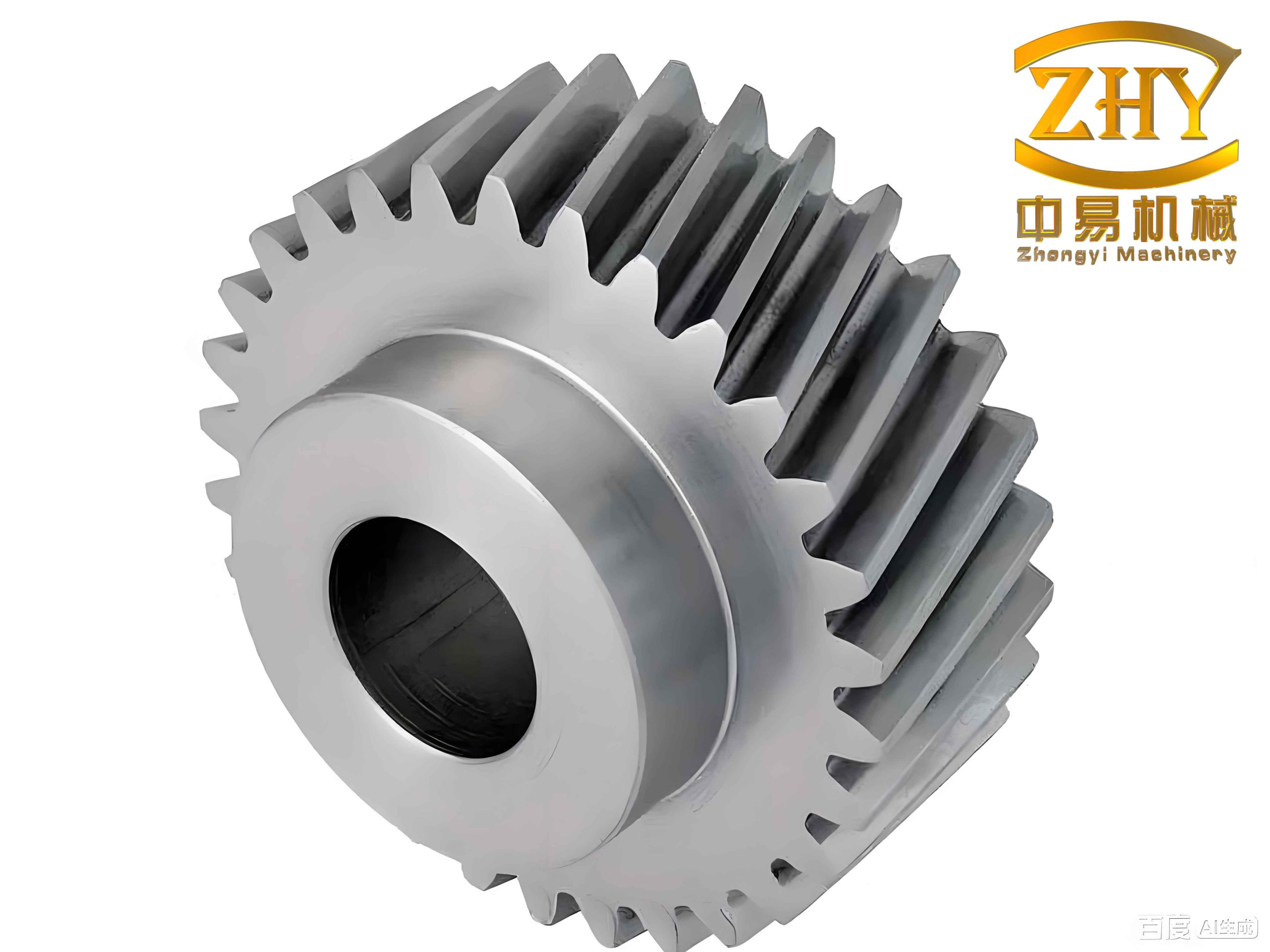
My work followed a complete numerical route. I first created a parametric model of a standard involute helical gear pair. I then performed static finite element analysis to obtain contact stress and root bending stress. After that, I imported the same helical gears into a dynamic simulation environment to obtain speed, meshing force, rotation angle, and transmission error. I used these results as the baseline for a genetic-algorithm-based multi-objective optimization. The optimization treated mass and transmission vibration as objectives, while contact stress and bending stress were treated as constraints. Finally, I rebuilt the optimized helical gears and repeated the static and dynamic simulations to verify that the new design was both lighter and quieter.
Parametric modeling of helical gears. I selected a standard involute helical gear pair as the research object. The basic parameters are listed in Table 1. The normal module, normal pressure angle, helix angle, tooth numbers, addendum coefficient, clearance coefficient, and face widths define the initial geometry. For helical gears, the normal plane parameters must be converted into the transverse plane before the involute profile can be generated correctly.
| Parameter | Symbol | Driving gear | Driven gear |
|---|---|---|---|
| Normal module (mm) | \(m_n\) | 2.5 | 2.5 |
| Normal pressure angle (deg) | \(\alpha_n\) | 20 | 20 |
| Reference helix angle (deg) | \(\beta\) | 14.84 | 14.84 |
| Number of teeth | \(z\) | 20 | 96 |
| Normal addendum coefficient | \(h_{an}^{*}\) | 1 | 1 |
| Normal clearance coefficient | \(c_n^{*}\) | 0.25 | 0.25 |
| Face width (mm) | \(b\) | 46 | 54 |
The transverse module is
$$m_t = \frac{m_n}{\cos\beta}.$$
The transverse pressure angle is
$$\tan\alpha_t = \frac{\tan\alpha_n}{\cos\beta}.$$
The addendum and dedendum are
$$h_a = h_{an}^{*}m_n,$$
$$h_f = \left(h_{an}^{*}+c_n^{*}\right)m_n.$$
The reference, tip, root, and base diameters are
$$d = m_t z,$$
$$d_a = d + 2h_a,$$
$$d_f = d – 2h_f,$$
$$d_b = d\cos\alpha_t.$$
For the involute geometry, I used the standard generation principle. If a straight line rolls without slipping on a base circle, any point on that line traces an involute. The involute equation in a Cartesian coordinate system can be written as
$$x = r_b\cos\phi + r_b\phi\sin\phi,$$
$$y = r_b\sin\phi – r_b\phi\cos\phi.$$
The involute polar angle relation is
$$\theta_k = \tan\alpha_k – \alpha_k,$$
$$\phi_k = \theta_k + \alpha_k = \tan\alpha_k.$$
In the three-dimensional modeling environment, I inserted an equation-driven curve to create the involute profile. The parametric equation that I used had the following form:
$$x = \frac{d_b}{2}\cos t + \frac{d_b}{2}t\sin t,$$
$$y = \frac{d_b}{2}\sin t – \frac{d_b}{2}t\cos t,$$
$$t \in [0,\pi/2].$$
I defined the root circle, base circle, reference circle, and tip circle as parameter-driven sketches. I then mirrored the involute curve, closed the tooth profile, extruded the body, cut the tooth space, and patterned the tooth around the gear axis. Because the model was parametric, changing the module, tooth number, helix angle, or face width automatically regenerated the helical gears. This was important for the later optimization because I needed to rebuild the helical gears quickly after the genetic algorithm produced new design variables.
Static finite element analysis of helical gears. Before static analysis, I simplified the full gear pair into a sector model containing only the meshing teeth. This reduced the computational cost and allowed a denser mesh near the contact zone. I exported the simplified assembly in Parasolid format and imported it into the finite element environment. The material properties were assigned as shown in Table 2.
| Property | Value |
|---|---|
| Elastic modulus | 206 GPa |
| Density | 7850 kg/m3 |
| Poisson ratio | 0.3 |
| Contact friction coefficient | 0.05 |
I used tetrahedral elements and refined the mesh in the contact region. The mesh contained approximately 175007 nodes and 101994 elements. The contact pair was defined as frictional contact because sliding occurs along the involute flanks during meshing. The driven helical gear was fixed in all degrees of freedom, and a torque was applied to the driving helical gear. The torque was calculated from the power and speed as
$$T = 9.55 \times 10^6 \frac{P}{n},$$
where \(P = 14.84\,\text{kW}\) and \(n = 970\,\text{r/min}\). The resulting torque was \(T = 145908\,\text{N}\cdot\text{mm}\).
After solving the static model, I obtained the contact stress distribution. The maximum contact stress from the finite element analysis was \(802.29\,\text{MPa}\). I also calculated the contact stress using the classical helical gear formula:
$$\sigma_H = Z_H Z_E Z_{\varepsilon} Z_{\beta}\sqrt{\frac{2KT_1}{bd_1^2}\frac{u+1}{u}}.$$
The classical parameters are summarized in Table 3, and the calculated contact stress was \(882.2\,\text{MPa}\). The finite element result was slightly lower than the classical result, which is expected because the classical formula is based on Hertz assumptions and tabulated coefficients, while the finite element method approximates the actual contact geometry and load distribution.
| Parameter | \(Z_H\) | \(Z_E\) | \(Z_{\varepsilon}\) | \(Z_{\beta}\) | \(K\) | \(u\) |
|---|---|---|---|---|---|---|
| Value | 2.43 | 189.8 | 0.784 | 0.983 | 2.15 | 4.8 |
The allowable contact stress was calculated as
$$[\sigma_H] = \frac{\sigma_{H\lim}Z_N Z_X Z_W Z_{LVR}}{S_H}.$$
Using \(\sigma_{H\lim}=1150\,\text{MPa}\), \(S_H=1.0\), \(Z_N=1.0\), \(Z_X=1.0\), \(Z_W=1.0\), and \(Z_{LVR}=0.92\), I obtained \([\sigma_H]=1058\,\text{MPa}\). Both the finite element and classical contact stresses were below this allowable value, so the initial helical gears satisfied the contact strength requirement.
For bending stress, I evaluated the root stress of both gears. The maximum root bending stress of the driving gear was \(275.66\,\text{MPa}\), and the maximum root bending stress of the driven gear was \(215.35\,\text{MPa}\). The classical bending stress formula for helical gears is
$$\sigma_F = \frac{2KT_1}{bd_1m}Y_{Fa}Y_{Sa}Y_{\varepsilon}Y_{\beta}.$$
The classical coefficients are listed in Table 4. The calculated driving gear bending stress was \(255.89\,\text{MPa}\), and the driven gear bending stress was \(229.61\,\text{MPa}\). The finite element values were close to the classical values, although the driving gear root stress was higher in the finite element result because the root fillet and load sharing were represented more explicitly.
| Parameter | \(K\) | \(Y_{Fa1}\) | \(Y_{Sa1}\) | \(Y_{Fa2}\) | \(Y_{Sa2}\) | \(Y_{\varepsilon}\) | \(Y_{\beta}\) |
|---|---|---|---|---|---|---|---|
| Value | 2.15 | 2.77 | 1.57 | 2.18 | 1.79 | 0.68 | 0.82 |
The allowable bending stress is
$$[\sigma_F] = \frac{\sigma_{F\lim}Y_N Y_X Y_{ST}}{S_F}.$$
Using \(\sigma_{F\lim}=340\,\text{MPa}\), \(S_F=1.25\), \(Y_N=1.0\), \(Y_X=0.99\), and \(Y_{ST}=2.0\), I obtained \([\sigma_F]=538.56\,\text{MPa}\). Both finite element bending stresses were below this value, confirming that the initial helical gears also satisfied the bending strength requirement.
Dynamic simulation of helical gears. I used a virtual prototyping approach to study the dynamic behavior of the helical gears. The parametric assembly was saved as Parasolid and imported into a dynamic simulation package. This format preserved the tooth surfaces more accurately than neutral formats and avoided loss of contact geometry. I defined revolute joints between each gear and the ground, and I defined a solid-to-solid contact between the meshing teeth. The driving helical gear was given a constant angular velocity of \(970\,\text{r/min}\), which is \(5820\,\text{deg/s}\). The driven helical gear was loaded with a step torque opposite to its rotation direction, with a magnitude of \(700358.4\,\text{N}\cdot\text{mm}\). The simulation time was \(0.5\,\text{s}\) with 500 steps.
For contact force calculation, I used the impact function method. The contact normal force is
$$F_n = K\delta^{e} + C\frac{d\delta}{dt},$$
where \(K\) is contact stiffness, \(\delta\) is penetration, \(e\) is the force exponent, and \(C\) is damping. Based on Hertz elastic contact theory, the contact stiffness for two cylinders with equivalent radius \(R\) and equivalent elastic modulus \(E\) is
$$K = \frac{4}{3}\sqrt{R}E.$$
For the original helical gears, the equivalent contact stiffness was \(K=698138.27\,\text{N/mm}\). The damping coefficient was \(50\,\text{N}\cdot\text{s/mm}\), the force exponent was \(1.5\), the dynamic friction coefficient was \(0.05\), the static friction coefficient was \(0.08\), and the penetration depth was \(0.1\,\text{mm}\). These parameters are summarized in Table 5.
| Dynamic contact parameter | Value |
|---|---|
| Contact stiffness \(K\) | 698138.27 N/mm |
| Damping coefficient \(C\) | 50 N s/mm |
| Force exponent \(e\) | 1.5 |
| Dynamic friction coefficient | 0.05 |
| Static friction coefficient | 0.08 |
| Penetration depth | 0.1 mm |
The speed simulation showed that the driving gear speed remained constant at \(5820\,\text{deg/s}\). The driven gear speed rose rapidly during start-up, fluctuated because of impact, and then settled around a stable mean. The theoretical driven speed was \(1212.5\,\text{deg/s}\), while the simulated mean was \(1210\,\text{deg/s}\), giving a relative error of \(0.2\%\). These results are shown in Table 6.
| Item | Theoretical value | Simulated mean | Relative error |
|---|---|---|---|
| Driving gear speed (deg/s) | 5820 | 5820 | 0% |
| Driven gear speed (deg/s) | 1212.5 | 1210 | 0.2% |
The theoretical meshing forces of a helical gear can be calculated from the torque and geometry. The tangential, radial, axial, and normal forces are
$$F_t = \frac{2T_1}{d_1},$$
$$F_r = F_t \frac{\tan\alpha_n}{\cos\beta},$$
$$F_a = F_t \tan\beta,$$
$$F_n = \frac{F_t}{\cos\alpha_n\cos\beta}.$$
I compared the theoretical forces with the stable simulation averages. The comparison is given in Table 7. The radial force error was \(7.5\%\), the tangential force error was \(3.3\%\), the axial force error was \(1.9\%\), and the normal force error was \(2.2\%\). These differences were acceptable and indicated that the dynamic model represented the real helical gears well.
| Force component | Theoretical value (N) | Simulated mean (N) | Relative error |
|---|---|---|---|
| Radial force | 2125 | 1964 | 7.5% |
| Tangential force | 5644 | 5836 | 3.3% |
| Axial force | 1495 | 1523 | 1.9% |
| Normal force | 6214 | 6352 | 2.2% |
Transmission error is one of the most useful indicators of dynamic performance in helical gears. It represents the difference between the actual rotation angle of the driven gear and its ideal rotation angle. I defined it as
$$TE = \theta_{B1} – \theta_{A1},$$
or equivalently as a displacement along the line of action:
$$TE = R_{bB1}\left(\theta_{B1} – \theta_{A1}\right).$$
I first checked the rotation angles after \(0.5\,\text{s}\). The driving gear rotated \(2910^\circ\), matching the theoretical value exactly. The driven gear rotated \(606.210^\circ\) in simulation and \(606.250^\circ\) theoretically, with a relative error of \(0.0066\%\). I then converted the driving gear angle into the theoretical driven gear angle using the transmission ratio and subtracted the actual driven angle. The stable transmission error varied between \(0.0188^\circ\) and \(0.0437^\circ\), giving a fluctuation amplitude of \(0.0249^\circ\). This amplitude served as the baseline vibration index for the original helical gears.
Genetic algorithm optimization. I selected a genetic algorithm because it is a population-based global search method. It does not require gradient information, it can handle nonlinear constraints, and it can search multiple regions of the design space simultaneously. The algorithm uses encoding, initial population generation, fitness evaluation, selection, crossover, and mutation. I used binary encoding for the design variables, tournament selection, a crossover probability of \(0.8\), a mutation probability of \(0.01\), and a population size of \(50\). The optimization ran for 102 generations. The algorithm workflow was designed so that each individual represented a complete set of helical gear parameters, and the fitness reflected both mass and vibration performance.
For the vibration objective, I reduced the helical gear pair to an equivalent mass-spring system along the line of action. The equivalent mass is
$$M_e = \frac{M_1M_2}{M_1+M_2} = \frac{J_1J_2}{J_1z_2^2 + J_2z_1^2}\frac{4\cos^2\beta}{m_n^2\cos^2\alpha_t}.$$
The equivalent mesh stiffness is
$$K_e = \frac{K_1K_2}{K_1+K_2} = \frac{\pi}{125}\frac{B_1B_2E_1E_2}{B_1E_1 + B_2E_2}.$$
The natural frequency of the equivalent system is
$$f_n = \frac{1}{2\pi}\sqrt{\frac{K_e}{M_e}}.$$
The mesh excitation frequency is
$$f = \frac{n_1z_1}{60}.$$
When the excitation frequency approaches the natural frequency, resonance occurs and vibration becomes severe. Therefore, I defined the vibration objective as maximizing the difference between the critical speed and the operating speed. The critical speed is
$$n_{cr} = \frac{60f_n}{z_1}.$$
To make all objectives minimization problems, I wrote the vibration objective as
$$f_1(x) = -\left(n_{cr} – n_1\right).$$
For the mass objective, I approximated the volume of each helical gear using the reference diameter and the shaft hole diameter:
$$V = \frac{\pi}{4}b\left(d^2 – d_p^2\right).$$
Thus, the total mass objective is
$$f_2(x) = \rho \left(V_1 + V_2\right) = \frac{\pi}{4}\rho\left[b_1\left(\frac{m_nz_1}{\cos\beta}\right)^2 + b_2\left(\frac{m_nz_2}{\cos\beta}\right)^2 – b_1d_{p1}^2 – b_2d_{p2}^2\right].$$
I combined the two objectives using a weighted sum. Before combining, I normalized each objective by its initial value:
$$f(x) = w_1\frac{f_1(x)}{f_1^{*}(x)} + w_2\frac{f_2(x)}{f_2^{*}(x)},$$
with \(w_1 = 0.5\) and \(w_2 = 0.5\). This gave equal importance to vibration reduction and mass reduction.
The design variables were the normal module, the driving gear tooth number, the driven gear tooth number, the helix angle, and the face width coefficient:
$$X = \left[m_n, z_1, z_2, \beta, \phi_d\right]^T.$$
The bounds and constraints are summarized in Table 8. The module was constrained between 2.5 and 6 mm. The helix angle was constrained between 8 and 15 degrees. The driving gear tooth number was constrained between 17 and 24 to avoid undercut and excessive size. The driven gear tooth number was constrained between 90 and 100 to keep the transmission ratio close to the original design. The face width coefficient was constrained between 0.4 and 0.9. In addition, the driven gear face width was set as \(b_2 = b_1 – 5\,\text{mm}\), reflecting the usual practice for helical gears.
| Constraint | Expression | Lower bound | Upper bound |
|---|---|---|---|
| Normal module | \(m_n\) | 2.5 mm | 6 mm |
| Helix angle | \(\beta\) | 8 deg | 15 deg |
| Driving tooth number | \(z_1\) | 17 | 24 |
| Driven tooth number | \(z_2\) | 90 | 100 |
| Face width coefficient | \(\phi_d\) | 0.4 | 0.9 |
| Face width relation | \(b_1 = b_2 + 5\) | — | — |
The performance constraints were based on contact and bending strength. The contact stress constraint was
$$g_H(x) = \sigma_H – 1058 \leq 0.$$
The driving gear bending stress constraint was
$$g_{F1}(x) = \sigma_{F1} – 539 \leq 0.$$
The driven gear bending stress constraint was
$$g_{F2}(x) = \sigma_{F2} – 475 \leq 0.$$
These constraints ensured that the optimized helical gears would not fail by surface pitting or root fracture.
The genetic algorithm produced a theoretical optimum of
$$X^{*} = \left[12.579^\circ, 2.502\,\text{mm}, 20.812, 91.273, 0.551\right]^T.$$
Because tooth numbers must be integers and the module should follow standard values, I rounded the result to
$$X = \left[12.58^\circ, 2.5\,\text{mm}, 21, 91, 0.55\right]^T.$$
The final objective value was approximately \(0.79\). The original and optimized parameters are compared in Table 9. The total mass of the helical gear pair decreased from \(15.68\,\text{kg}\) to \(9.47\,\text{kg}\), a reduction of \(39.6\%\). The vibration objective changed from \(-937.37\) to \(-941.23\), indicating that the difference between the operating speed and the critical speed increased and the transmission became more stable.
| Parameter | Original | Optimized |
|---|---|---|
| Normal module \(m_n\) (mm) | 2.5 | 2.5 |
| Driving gear tooth number \(z_1\) | 20 | 21 |
| Driven gear tooth number \(z_2\) | 96 | 91 |
| Face width coefficient \(\phi_d\) | 0.87 | 0.55 |
| Helix angle \(\beta\) (deg) | 14.84 | 12.58 |
| Mass (kg) | 15.68 | 9.47 |
| Vibration objective \(f_1(x)\) | -937.37 | -941.23 |
Verification of the optimized helical gears. I rebuilt the optimized helical gears using the same parametric modeling procedure. I then repeated the static finite element analysis with the same material, contact definition, mesh refinement strategy, and boundary conditions. The optimized contact stress was \(790.56\,\text{MPa}\), compared with \(802.29\,\text{MPa}\) for the original helical gears. The maximum root bending stress of the driving gear decreased from \(275.66\,\text{MPa}\) to \(212.2\,\text{MPa}\). The maximum root bending stress of the driven gear decreased from \(215.35\,\text{MPa}\) to \(169.44\,\text{MPa}\). All optimized stresses remained below the allowable limits. The static verification results are shown in Table 10.
| Stress item | Original (MPa) | Optimized (MPa) | Relative change |
|---|---|---|---|
| Maximum contact stress | 802.29 | 790.56 | 1.5% |
| Driving gear root bending stress | 275.66 | 212.2 | 23.0% |
| Driven gear root bending stress | 215.35 | 169.44 | 21.3% |
| Allowable contact stress | 1058 | 1058 | — |
| Allowable driving bending stress | 539 | 539 | — |
| Allowable driven bending stress | 475 | 475 | — |
I then repeated the dynamic simulation for the optimized helical gears. Because the tooth geometry and face width changed, the contact stiffness and the resisting torque also changed. The new contact stiffness was \(K=623338.67\,\text{N/mm}\), and the new resisting torque was \(632268\,\text{N}\cdot\text{mm}\). All other contact parameters were kept the same. The optimized meshing force averages are compared with the original values in Table 11.
| Force component | Original mean (N) | Optimized mean (N) | Relative change |
|---|---|---|---|
| Radial force | 1964 | 2270 | 15.5% |
| Tangential force | 5836 | 5486 | 5.9% |
| Axial force | 1523 | 1237 | 19.5% |
| Normal force | 6352 | 6068 | 4.5% |
The force changes reflected the new tooth geometry. The normal force decreased, which is favorable for bearing load and vibration excitation. The axial force also decreased because the helix angle was reduced. The radial force increased, but the overall dynamic response still improved, as shown by the transmission error.
I also checked the rotation angles of the optimized helical gears. The driving gear rotated \(2910^\circ\), matching the theoretical value. The driven gear rotated \(671.500^\circ\) in simulation and \(671.539^\circ\) theoretically, with a relative error of \(0.0058\%\). The optimized transmission error varied between \(0.0278^\circ\) and \(0.0499^\circ\), giving a fluctuation amplitude of \(0.0221^\circ\). The original amplitude was \(0.0249^\circ\). Therefore, the optimized helical gears reduced the transmission error amplitude by \(11.2\%\). This confirmed that the optimized helical gears are not only lighter but also dynamically smoother. The transmission error comparison is given in Table 12.
| Transmission error item | Original | Optimized | Relative change |
|---|---|---|---|
| Upper fluctuation limit (deg) | 0.0437 | 0.0499 | 14.1% |
| Lower fluctuation limit (deg) | 0.0188 | 0.0278 | 47.9% |
| Fluctuation amplitude (deg) | 0.0249 | 0.0221 | 11.2% |
Interpretation of the optimization results. The genetic algorithm found a balanced design for the helical gears. The tooth numbers changed only slightly, but the face width coefficient and helix angle changed more clearly. The face width coefficient decreased from 0.87 to 0.55, which reduced the volume and mass of the helical gears. The helix angle decreased from \(14.84^\circ\) to \(12.58^\circ\), which reduced axial force and affected the contact ratio and mesh stiffness. The module remained at \(2.5\,\text{mm}\), so the overall tooth size stayed within a standard and manufacturable range. The driving gear tooth number increased from 20 to 21, while the driven gear tooth number decreased from 96 to 91. These changes kept the transmission ratio close to the original value while improving the dynamic objective.
The static verification showed that the optimized helical gears maintained sufficient safety margins. The contact stress decreased slightly, and the root bending stresses decreased significantly. This means that the mass reduction did not come at the expense of strength. The dynamic verification showed that the normal meshing force decreased and the transmission error amplitude decreased. Lower meshing force and lower transmission error are both beneficial for reducing vibration and noise in helical gears.
Further discussion of helical gears vibration. Vibration in helical gears comes from internal and external excitation. Internal excitation includes tooth impact, mesh stiffness variation, transmission error, and profile deviation. External excitation includes load fluctuation, shaft misalignment, and bearing clearance. In my model, I focused on the internal excitation caused by the gear pair itself. I used transmission error as the main dynamic indicator because it directly reflects the geometric and elastic compatibility of the meshing process. A smaller transmission error amplitude means that the driven gear follows the ideal motion more closely, so the impact at tooth engagement and disengagement is weaker.
I also considered the effect of equivalent mesh stiffness. The natural frequency of the helical gear pair depends on the ratio of mesh stiffness to equivalent mass. If the natural frequency is close to the mesh excitation frequency, resonance can amplify vibration. By changing the tooth number, helix angle, and face width, the genetic algorithm shifted the critical speed away from the operating speed. The vibration objective became more negative, which means that the absolute difference between the critical speed and the operating speed increased. This is a simple but effective way to reduce the risk of resonance in helical gears.
Lightweight design of helical gears. The mass objective was based on the reference diameter and face width. This is a common approximation because the exact tooth volume is complex and depends on the involute profile, fillets, and hub geometry. Even with this approximation, the relative mass reduction was large. The optimized helical gears used less material, which lowers raw material cost, machining time, and rotational inertia. Lower rotational inertia also improves dynamic response because the gear pair requires less torque to accelerate and produces less kinetic energy during impact. In this sense, lightweight design and vibration reduction are not separate goals; they reinforce each other in helical gears.
Limitations and improvements. The mass model did not include the hub, web, keyway, or shaft. In a real helical gear, these features contribute to mass and stiffness. The dynamic model did not include manufacturing error, assembly error, bearing compliance, or thermal deformation. In actual operation, these factors can change the contact pattern and transmission error. The contact model used Hertz theory, which assumes elastic deformation and ignores friction heating and lubrication effects. Future work could include a more detailed hub and web geometry, measured profile deviations, a flexible shaft model, and thermo-mechanical coupling. A faster optimization algorithm could also be used to reduce the computation time of the genetic algorithm.
Conclusion. I studied lightweight design and vibration reduction for helical gears using parametric modeling, static finite element analysis, dynamic simulation, and genetic algorithm optimization. The initial helical gears satisfied contact and bending strength requirements. The dynamic simulation produced speed, meshing force, and transmission error results that agreed well with theoretical values. I then formulated a multi-objective optimization problem with mass and vibration as objectives and contact and bending strength as constraints. The genetic algorithm reduced the mass of the helical gear pair from \(15.68\,\text{kg}\) to \(9.47\,\text{kg}\), a reduction of \(39.6\%\). The optimized helical gears also reduced the transmission error fluctuation amplitude from \(0.0249^\circ\) to \(0.0221^\circ\), a reduction of \(11.2\%\). Static verification showed that the optimized contact stress and root bending stresses remained below allowable limits. Dynamic verification showed that the normal meshing force decreased and the transmission became smoother. Therefore, the optimized helical gears achieved both lightweight construction and reduced vibration while preserving strength. The method provides a practical route for designing quieter and lighter helical gears in mechanical transmission systems.