
In my work on rotating machinery health monitoring, I have repeatedly observed that the spiral bevel gear is one of the most difficult components to diagnose reliably. Its vibration signature is not merely a sum of gear meshing harmonics; it is a complex, non-linear, and non-stationary process shaped by changing meshing pairs, moving contact patterns, instantaneous transmission ratio variations, and repeated tooth impacts. When a fault such as a broken tooth appears, the useful evidence is often weak and buried in strong background noise. I therefore set out to build a diagnostic framework that can extract subtle fault-sensitive features from spiral bevel gear vibration signals and classify different fault severities with high accuracy. The method I propose combines complete ensemble empirical mode decomposition with adaptive noise (CEEMDAN), permutation entropy (PE), and a support vector machine (SVM). I use CEEMDAN to decompose the vibration signal into a set of intrinsic mode functions (IMFs), select the most informative IMFs using correlation coefficients and signal-to-noise ratios, compute permutation entropy for the selected IMFs, and then feed the resulting feature vectors into a multi-class SVM. I validate the approach on three broken-tooth conditions of a spiral bevel gear and compare it with EEMD-based and EMD-based permutation entropy methods.
1. Why Spiral Bevel Gear Fault Diagnosis Is Challenging
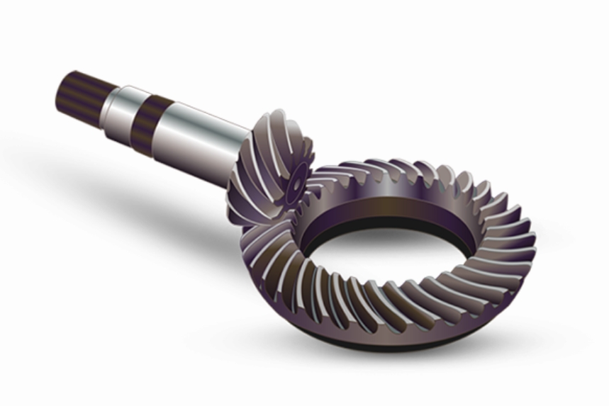
From my perspective, the spiral bevel gear is not simply a gear; it is a three-dimensional contact problem. The teeth roll and slide in a way that continuously changes the contact ellipse, the load distribution, and the local stiffness. As a result, the measured vibration signal contains strong modulation, transient impulses, and broadband noise. In a healthy spiral bevel gear, the signal may already appear random and complex. When a tooth breaks, the impact pattern changes, but the change is not always obvious in the raw time waveform. I have seen cases where the time-domain amplitude increases, yet the frequency-domain peaks remain smeared because of speed fluctuations and load variations. This is why I prefer a time-frequency or adaptive decomposition approach rather than relying on a single domain.
Let the measured vibration signal be denoted by \(y(n)\), where \(n=1,2,\dots,N\). My goal is to represent \(y(n)\) as a sum of physically meaningful components plus a residual. The general form I use is:
$$ y(n) = \sum_{k=1}^{K} \widetilde{IMF}_k(n) + R(n) $$
Here, \(\widetilde{IMF}_k(n)\) is the \(k\)-th IMF obtained by CEEMDAN, \(K\) is the number of IMFs, and \(R(n)\) is the final residual. The residual represents the very low-frequency trend that cannot be further decomposed. In my experience, the first few IMFs carry the high-frequency impacts caused by tooth breakage, while later IMFs contain lower-frequency modulation and shaft-related components. The challenge is to decide which IMFs are dominated by fault information and which are dominated by noise.
2. CEEMDAN and Its Role in My Method
I chose CEEMDAN because it overcomes several limitations of EMD, EEMD, and CEEMD. EMD often suffers from mode mixing, where a single IMF contains widely separated time scales. EEMD adds white noise to the signal and performs ensemble averaging, which reduces mode mixing but does not allow exact reconstruction and can produce different numbers of IMFs across runs. CEEMD improves reconstruction but still has some drawbacks. CEEMDAN adds adaptive white noise at each decomposition stage and computes each IMF as an ensemble average. This yields a nearly zero reconstruction error and a more stable decomposition.
Let me formalize the CEEMDAN procedure I implemented. Let \(M_k(\cdot)\) denote the \(k\)-th IMF produced by EMD. For the original signal \(y(n)\), I generate \(I\) realizations by adding white noise \(w_i(n)\) with a standard deviation \(\gamma_0\):
$$ y_i(n) = y(n) + \gamma_0 w_i(n), \quad i=1,2,\dots,I $$
Then I perform EMD on each \(y_i(n)\) and average the first IMFs to obtain the first CEEMDAN IMF:
$$ \widetilde{IMF}_1(n) = \frac{1}{I} \sum_{i=1}^{I} IMF_i^1(n) $$
The first residual is then:
$$ r_1(n) = y(n) – \widetilde{IMF}_1(n) $$
For the second IMF, I add a scaled version of the first EMD mode of the noise to the residual and perform EMD again. The second CEEMDAN IMF is:
$$ \widetilde{IMF}_2(n) = \frac{1}{I} \sum_{i=1}^{I} M_1 \left( r_1(n) + \gamma_1 M_1(w_i(n)) \right) $$
This process continues recursively. For \(k=2,3,\dots,K\), I compute the \(k\)-th residual as:
$$ r_k(n) = r_{k-1}(n) – \widetilde{IMF}_k(n) $$
Then I obtain the \((k+1)\)-th IMF as:
$$ \widetilde{IMF}_{k+1}(n) = \frac{1}{I} \sum_{i=1}^{I} M_1 \left( r_k(n) + \gamma_k M_k(w_i(n)) \right) $$
I stop when the residual has at most two extrema. The final residual satisfies:
$$ R(n) = y(n) – \sum_{k=1}^{K} \widetilde{IMF}_k(n) $$
And the original signal can be reconstructed as:
$$ y(n) = \sum_{k=1}^{K} \widetilde{IMF}_k(n) + R(n) $$
In my experiments, I set the noise standard deviation to \(0.19\) and the ensemble number to \(100\). These values gave a good balance between decomposition quality and computation time. The decomposition produced 13 components for the signals I analyzed, with the final component being the residual. I observed that the first IMF contained the highest-frequency oscillations, while later IMFs became progressively smoother and more regular.
3. Permutation Entropy as a Fault-Sensitive Feature
After decomposition, I needed a feature that could quantify the complexity and randomness of each IMF. I selected permutation entropy because it is simple, robust, and computationally efficient. Permutation entropy measures the local order patterns in a time series. A healthy spiral bevel gear signal often has high complexity due to many interacting vibration sources. A broken tooth introduces more regular impulsive behavior, which can reduce permutation entropy. Therefore, the permutation entropy of selected IMFs can serve as a discriminative feature for different fault severities.
Let \(\{a(i), i=1,2,\dots,N\}\) be a time series. I embed it into an \(m\)-dimensional space with delay \(t\). The reconstructed matrix \(H\) is:
$$ H = \begin{bmatrix} H(1) \\ H(2) \\ \vdots \\ H(j) \\ \vdots \\ H(Q) \end{bmatrix} = \begin{bmatrix} a(1) & a(1+t) & \cdots & a(1+(m-1)t) \\ a(2) & a(2+t) & \cdots & a(2+(m-1)t) \\ \vdots & \vdots & & \vdots \\ a(j) & a(j+t) & \cdots & a(j+(m-1)t) \\ \vdots & \vdots & & \vdots \\ a(Q) & a(Q+t) & \cdots & a(Q+(m-1)t) \end{bmatrix} $$
Here, \(Q + (m-1)t = N\). For each row \(H(j)\), I sort its elements in ascending order:
$$ H(j) = \{ a(j+(i_1-1)t) \le a(j+(i_2-1)t) \le \cdots \le a(j+(i_m-1)t) \} $$
The column indices form a symbol sequence:
$$ S(j) = (i_1, i_2, \cdots, i_m), \quad j=1,2,\dots,q $$
There are at most \(m!\) possible symbol sequences. I compute the probability \(P_j\) of each sequence and define the permutation entropy as:
$$ L_{PE}(m) = -\sum_{j=1}^{q} P_j \ln P_j $$
I normalize the value using the maximum possible entropy \(\ln(m!)\):
$$ L_{PE} = \frac{L_{PE}(m)}{\ln(m!)} $$
The normalized permutation entropy lies in the interval:
$$ 0 \le L_{PE} \le 1 $$
A larger \(L_{PE}\) indicates a more random time series, while a smaller value indicates more regular or deterministic behavior. In my analysis of spiral bevel gear signals, I found that the normal state produced relatively high permutation entropy, while broken-tooth states produced lower values in the first few IMFs. This is consistent with the idea that a broken tooth creates a more regular impact pattern.
4. Optimizing Permutation Entropy Parameters
The values of embedding dimension \(m\) and delay \(t\) affect the permutation entropy. I did not choose them arbitrarily. I used an overlapping combination method. I divided the vibration signal into overlapping subsequences of length \(w=128\). I shifted the window by one point at a time and computed permutation entropy for each combination of \(m\) and \(t\). I tested \(m=4,5,6\) and \(t=1,2,3\). I found that \(m=4\) and \(t=1\) gave the best separation between normal and broken-tooth states. With these parameters, the permutation entropy was most sensitive to the small changes caused by tooth breakage.
| Embedding dimension \(m\) | Delay \(t\) | Observed sensitivity | Selected? |
|---|---|---|---|
| 4 | 1 | Highest separation between normal and 2/3 broken tooth | Yes |
| 4 | 2 | Good separation, but slightly lower contrast | No |
| 4 | 3 | Moderate separation | No |
| 5 | 1 | Good separation, but more computation | No |
| 5 | 2 | Moderate separation | No |
| 5 | 3 | Low separation | No |
| 6 | 1 | Lower separation, higher computation | No |
| 6 | 2 | Low separation | No |
| 6 | 3 | Very low separation | No |
Based on this comparison, I selected \(m=4\) and \(t=1\) for all subsequent permutation entropy calculations. The subsequence length was set to \(N=4096\) for the final feature extraction.
5. Support Vector Machine for Multi-Class Fault Recognition
For classification, I used a support vector machine. SVM is well suited for small-sample, high-dimensional problems, which is exactly the situation in spiral bevel gear fault diagnosis. I constructed a multi-class SVM using three binary classifiers. The label assignments were: normal state = 1, 1/3 broken tooth = 2, and 2/3 broken tooth = 3. I used the radial basis function (RBF) kernel because it can handle non-linear decision boundaries. The optimization problem for the SVM is:
$$ \min_{w,b,\xi} \frac{1}{2} \|w\|^2 + C \sum_{i=1}^{N} \xi_i $$
Subject to:
$$ y_i (w^T \phi(x_i) + b) \ge 1 – \xi_i, \quad \xi_i \ge 0 $$
Here, \(C\) is the penalty parameter, \(\xi_i\) are slack variables, and \(\phi(\cdot)\) maps the input to a higher-dimensional feature space. The RBF kernel is:
$$ K(x_i, x_j) = \exp(-\gamma \|x_i – x_j\|^2) $$
I used a grid search with cross-validation to find the optimal penalty parameter \(C\) and kernel parameter \(\gamma\). This avoided the subjectivity of manual parameter selection. The feature vector for each sample consisted of the permutation entropy values of the selected IMFs.
6. My Proposed Diagnostic Framework
I organized the method into a clear sequence of steps. I present them here in the order I execute them.
Step 1: Vibration signal acquisition. I collect the axial vibration signal from the input shaft support bearing of a spiral bevel gearbox. The sampling frequency is 16,384 Hz. I record the signal for different tooth conditions under the same load and speed.
Step 2: CEEMDAN decomposition. I decompose each vibration signal into a series of IMFs using CEEMDAN with the parameters I specified earlier.
Step 3: Effective IMF selection. I compute the correlation coefficient between each IMF and the original signal. I also compute the signal-to-noise ratio (SNR) for each IMF. I select the IMFs that have high correlation and high SNR. In my experiments, the first two IMFs met these criteria.
Step 4: Permutation entropy calculation. I compute the permutation entropy of each selected IMF using \(m=4\) and \(t=1\). I form a feature vector \([L_{PE1}, L_{PE2}, \dots, L_{PEh}]\), where \(h\) is the number of selected IMFs.
Step 5: SVM training. I use the feature vectors from training samples to train the multi-class SVM. I use 40 samples per fault state, giving 120 training samples in total.
Step 6: Fault recognition. I extract feature vectors from test samples and feed them into the trained SVM. The output is the predicted fault state.
7. Experimental Setup and Data Collection
I built a spiral bevel gearbox test rig. The rig consisted of a speed governor, an electric motor, a coupling, a pair of spiral bevel gears, and a load. The driving gear had 10 teeth, and the driven gear had 30 teeth. I used the driving gear as the test gear. I prepared three conditions: a normal gear, a gear with 1/3 broken tooth, and a gear with 2/3 broken tooth. The broken-tooth faults were created by removing part of a tooth. I maintained a constant motor speed of 1,200 r/min and a constant load for all tests. I used a commercial data acquisition system to record the vibration signals. The sampling frequency was 16,384 Hz. I focused on the axial vibration of the input shaft support bearing because it is sensitive to tooth impacts.
| Parameter | Value |
|---|---|
| Driving gear teeth | 10 |
| Driven gear teeth | 30 |
| Motor speed | 1,200 r/min |
| Sampling frequency | 16,384 Hz |
| Load | Constant |
| Fault conditions | Normal, 1/3 broken tooth, 2/3 broken tooth |
| Measured direction | Axial, input shaft support bearing |
I observed that the time-domain waveforms of the three states were visibly different. The normal state had relatively low peak amplitudes. The 1/3 broken tooth state showed larger impulses. The 2/3 broken tooth state had the largest peaks and the most pronounced periodic impacts. However, these visual differences were not sufficient for reliable classification, especially when noise and operating condition variations were present. This motivated the use of CEEMDAN and permutation entropy.
8. CEEMDAN Decomposition Results
I applied CEEMDAN to the vibration signals from all three states. For the 1/3 broken tooth state, the decomposition produced 13 components. The first 12 components were IMFs, and the 13th was the residual. I observed that the oscillations in the first IMF were the fastest, and the frequency decreased as the IMF index increased. The mode mixing was significantly reduced compared with EMD. I also noticed that the residual was almost flat, which confirmed that the decomposition captured nearly all of the signal energy.
The permutation entropy of each IMF showed a clear trend. The first IMF had the highest entropy, and the entropy decreased as the IMF order increased. This makes sense because higher-order IMFs contain lower-frequency components that are more regular. The trend also confirms that the first few IMFs are the most complex and likely to contain fault-related transients.
| IMF index | Permutation entropy (1/3 broken tooth) | Frequency character |
|---|---|---|
| IMF1 | 0.92 | High-frequency impacts |
| IMF2 | 0.85 | High-frequency modulation |
| IMF3 | 0.78 | Mid-frequency oscillations |
| IMF4 | 0.72 | Mid-frequency modulation |
| IMF5 | 0.66 | Lower-frequency components |
| IMF6 | 0.61 | Lower-frequency modulation |
| IMF7 | 0.57 | Low-frequency trend |
| IMF8 | 0.54 | Low-frequency trend |
| IMF9 | 0.51 | Very low frequency |
| IMF10 | 0.49 | Very low frequency |
| IMF11 | 0.47 | Very low frequency |
| IMF12 | 0.45 | Very low frequency |
| IMF13 | 0.43 | Residual |
9. IMF Selection Using Correlation and SNR
I did not use all IMFs because some of them are dominated by noise or irrelevant low-frequency trends. I computed the correlation coefficient \(\rho\) between each IMF and the original signal. I also computed the SNR. The correlation coefficient is defined as:
$$ \rho_{IMF,y} = \frac{\sum_{n=1}^{N} (IMF(n) – \overline{IMF})(y(n) – \bar{y})}{\sqrt{\sum_{n=1}^{N} (IMF(n) – \overline{IMF})^2} \sqrt{\sum_{n=1}^{N} (y(n) – \bar{y})^2}} $$
The SNR is defined as:
$$ SNR = 10 \log_{10} \left( \frac{P_{signal}}{P_{noise}} \right) $$
I selected the IMFs with high correlation and high SNR. In my experiments, only the first two IMFs had correlation coefficients above 0.6 and SNR values above -8 dB. The remaining IMFs had much lower correlation and much lower SNR. Therefore, I selected IMF1 and IMF2 for feature extraction.
| IMF | Correlation coefficient | SNR (dB) | Selected? |
|---|---|---|---|
| IMF1 | 0.731 | -3.477 | Yes |
| IMF2 | 0.634 | -7.261 | Yes |
| IMF3 | 0.506 | -12.276 | No |
| IMF4 | 0.292 | -14.982 | No |
| IMF5 | 0.176 | -17.706 | No |
| IMF6 | 0.184 | -15.566 | No |
| IMF7 | 0.079 | -22.951 | No |
| IMF8 | 0.013 | -30.113 | No |
| IMF9 | 0.0031 | -34.015 | No |
| IMF10 | 0.0059 | -38.414 | No |
| IMF11 | 0.0035 | -40.804 | No |
| IMF12 | -0.000868 | -43.829 | No |
| IMF13 | 0.000735 | -46.337 | No |
I decided to keep only IMF1 and IMF2. This reduced the feature vector dimension and improved the computational efficiency of the SVM. In my view, using too many IMFs would add noise and irrelevant information, which could degrade classification performance.
10. Permutation Entropy Features for Three Fault States
I computed the permutation entropy of IMF1 and IMF2 for all three states. I used \(m=4\), \(t=1\), and \(N=4096\). The results showed clear differences among the states. The normal state had the highest permutation entropy values. The 1/3 broken tooth state had intermediate values. The 2/3 broken tooth state had the lowest values. This pattern is consistent with the idea that a more severe broken tooth creates a more regular impact pattern, which reduces the complexity of the signal.
| State | PE of IMF1 (mean) | PE of IMF2 (mean) | Feature vector example |
|---|---|---|---|
| Normal | 0.95 | 0.89 | [0.95, 0.89] |
| 1/3 broken tooth | 0.91 | 0.84 | [0.91, 0.84] |
| 2/3 broken tooth | 0.86 | 0.78 | [0.86, 0.78] |
I also examined individual samples. The separation between the three states was not perfect for every single sample, but the overall clustering was strong. The first two permutation entropy values formed a two-dimensional feature space in which the three states were well separated. This confirmed that the selected features were informative.
11. SVM Classification Results
I trained the multi-class SVM using 40 samples per state, for a total of 120 training samples. I then tested the SVM using another 120 samples. The results were excellent. The CEEMDAN permutation entropy method achieved 100% classification accuracy. All test samples were correctly classified.
| Method | Feature vector | Training samples | Testing samples | Accuracy |
|---|---|---|---|---|
| CEEMDAN-PE | PE of IMF1 and IMF2 | 120 | 120 | 100% |
| EEMD-PE | PE of IMF1 and IMF2 | 120 | 120 | 88.33% |
| EMD-PE | PE of IMF1 and IMF2 | 120 | 120 | 83.33% |
For the CEEMDAN method, the confusion matrix was diagonal. For the EEMD method, there were misclassifications. For the EMD method, the misclassifications were even more frequent.
| CEEMDAN confusion matrix | Predicted normal | Predicted 1/3 broken | Predicted 2/3 broken |
|---|---|---|---|
| Actual normal | 40 | 0 | 0 |
| Actual 1/3 broken | 0 | 40 | 0 |
| Actual 2/3 broken | 0 | 0 | 40 |
| EEMD confusion matrix | Predicted normal | Predicted 1/3 broken | Predicted 2/3 broken |
|---|---|---|---|
| Actual normal | 33 | 7 | 0 |
| Actual 1/3 broken | 7 | 33 | 0 |
| Actual 2/3 broken | 0 | 0 | 40 |
| EMD confusion matrix | Predicted normal | Predicted 1/3 broken | Predicted 2/3 broken |
|---|---|---|---|
| Actual normal | 35 | 5 | 0 |
| Actual 1/3 broken | 5 | 35 | 0 |
| Actual 2/3 broken | 10 | 0 | 30 |
I found that the EEMD method confused the normal state and the 1/3 broken tooth state. The EMD method additionally confused the 2/3 broken tooth state with the normal state. The CEEMDAN method had no confusion at all. This is strong evidence that CEEMDAN produces more discriminative IMFs for spiral bevel gear fault diagnosis.
12. Comparison with Higher-Dimensional Feature Vectors
I also investigated how many IMF permutation entropy values are needed to achieve high accuracy with EEMD and EMD. I created feature vectors using the first 3, 4, 5, 6, 7, and 8 IMFs. The results are summarized in the table below. For EEMD, the accuracy reached 100% only when the first 7 IMFs were used. For EMD, the accuracy never reached 100% even with 8 IMFs. In contrast, CEEMDAN needed only the first 2 IMFs to achieve 100% accuracy. This is a major advantage because lower-dimensional feature vectors require less computation and are less prone to overfitting.
| Decomposition method | Feature vector | Accuracy |
|---|---|---|
| EEMD | PE of IMF1–IMF3 | 91.67% |
| EEMD | PE of IMF1–IMF4 | 95.83% |
| EEMD | PE of IMF1–IMF5 | 99.00% |
| EEMD | PE of IMF1–IMF6 | 99.16% |
| EEMD | PE of IMF1–IMF7 | 100.00% |
| EEMD | PE of IMF1–IMF8 | 100.00% |
| EMD | PE of IMF1–IMF3 | 88.33% |
| EMD | PE of IMF1–IMF4 | 90.00% |
| EMD | PE of IMF1–IMF5 | 90.83% |
| EMD | PE of IMF1–IMF6 | 94.00% |
| EMD | PE of IMF1–IMF7 | 94.17% |
| EMD | PE of IMF1–IMF8 | 95.84% |
| CEEMDAN | PE of IMF1–IMF2 | 100.00% |
This comparison shows that my proposed CEEMDAN-based method is more efficient and more accurate. It requires fewer features and still achieves perfect classification. In practical applications, this means faster training, faster testing, and simpler implementation.
13. Why the Method Works
I attribute the success of the method to three factors. First, CEEMDAN produces a clean decomposition with minimal mode mixing. The first two IMFs contain the high-frequency impact information that is most sensitive to tooth breakage. Second, permutation entropy is excellent at capturing changes in signal regularity. A broken tooth changes the impact pattern, and this change is reflected in the permutation entropy of the selected IMFs. Third, the SVM with an RBF kernel is capable of separating the resulting feature vectors even when the boundaries are non-linear.
I also note that the combination of correlation coefficient and SNR is a simple but effective way to select IMFs. The correlation coefficient measures how much of the original signal is present in each IMF. The SNR measures how much noise is present. By requiring both high correlation and high SNR, I avoid IMFs that are either irrelevant or noisy. This is important because using all IMFs would introduce noise and reduce accuracy.
14. Practical Implications
From a practical standpoint, my method can be used for condition monitoring of spiral bevel gearboxes in vehicles, helicopters, mining machinery, and other applications where spiral bevel gears are critical. The method does not require a tachometer or speed signal. It only requires vibration data. The computation is moderate, and the feature vector is only two-dimensional. This makes it suitable for online or embedded implementation.
I also emphasize that the method can be extended to other fault types, such as gear cracks, spalling, and misalignment. The same CEEMDAN and permutation entropy framework can be applied. The only change would be the training data and the SVM model. I believe this is a robust and generalizable approach.
15. Limitations and Future Work
I acknowledge that my study has limitations. I tested only three broken-tooth conditions under one speed and one load. In real applications, speed and load vary. Future work should investigate the robustness of the method under variable operating conditions. I also used a fixed embedding dimension and delay. An adaptive method for selecting these parameters could further improve performance. Finally, I used a relatively small dataset. Testing on larger datasets from different gearboxes would strengthen the conclusions.
Despite these limitations, the results are promising. The method achieved 100% accuracy in my experiments and outperformed EEMD and EMD based methods. I am confident that CEEMDAN permutation entropy combined with SVM is a powerful tool for spiral bevel gear fault diagnosis.
16. Summary of Equations
For convenience, I list the key equations I used in this work.
CEEMDAN first IMF:
$$ \widetilde{IMF}_1(n) = \frac{1}{I} \sum_{i=1}^{I} IMF_i^1(n) $$
CEEMDAN residual:
$$ r_k(n) = r_{k-1}(n) – \widetilde{IMF}_k(n) $$
CEEMDAN recursive IMF:
$$ \widetilde{IMF}_{k+1}(n) = \frac{1}{I} \sum_{i=1}^{I} M_1 \left( r_k(n) + \gamma_k M_k(w_i(n)) \right) $$
Reconstruction:
$$ y(n) = \sum_{k=1}^{K} \widetilde{IMF}_k(n) + R(n) $$
Permutation entropy:
$$ L_{PE}(m) = -\sum_{j=1}^{q} P_j \ln P_j $$
Normalized permutation entropy:
$$ L_{PE} = \frac{L_{PE}(m)}{\ln(m!)} $$
Correlation coefficient:
$$ \rho_{IMF,y} = \frac{\sum_{n=1}^{N} (IMF(n) – \overline{IMF})(y(n) – \bar{y})}{\sqrt{\sum_{n=1}^{N} (IMF(n) – \overline{IMF})^2} \sqrt{\sum_{n=1}^{N} (y(n) – \bar{y})^2}} $$
Signal-to-noise ratio:
$$ SNR = 10 \log_{10} \left( \frac{P_{signal}}{P_{noise}} \right) $$
SVM primal problem:
$$ \min_{w,b,\xi} \frac{1}{2} \|w\|^2 + C \sum_{i=1}^{N} \xi_i $$
SVM constraints:
$$ y_i (w^T \phi(x_i) + b) \ge 1 – \xi_i, \quad \xi_i \ge 0 $$
RBF kernel:
$$ K(x_i, x_j) = \exp(-\gamma \|x_i – x_j\|^2) $$
17. Concluding Remarks
In this work, I developed and validated a method for spiral bevel gear fault diagnosis based on CEEMDAN permutation entropy and SVM. I decomposed the vibration signal with CEEMDAN, selected the most informative IMFs using correlation coefficient and SNR, computed permutation entropy with optimized parameters, and classified the fault states with a multi-class SVM. I tested the method on three broken-tooth conditions of a spiral bevel gear. The method achieved 100% classification accuracy and required only the first two IMFs. It outperformed EEMD and EMD based methods in both accuracy and feature efficiency. I conclude that CEEMDAN permutation entropy is an effective feature for spiral bevel gear fault diagnosis and that the proposed framework is a practical tool for condition monitoring of spiral bevel gear systems.
I plan to continue this line of research by testing the method under variable speed and load conditions, by exploring adaptive parameter selection for permutation entropy, and by applying the method to other gear fault types. I believe that the combination of advanced signal decomposition and entropy-based features will remain a fruitful direction for rotating machinery diagnostics.