
I approach the modeling, simulation, additive manufacturing, and inspection of a matched pair of spiral bevel gears from a first-principles perspective. My central aim is to make the spiral bevel gear model both accurate and efficient, so that the resulting geometry can be used for motion simulation, rapid prototyping, and coordinate measurement. I base the entire workflow on spherical involute formation theory, because the spherical involute provides a natural description of the tooth surface of a spiral bevel gear when the motion is considered on a sphere centered at the cone apex. Instead of relying only on approximate tooth profiles, I generate discrete tooth-surface point coordinates, fit those points into smooth surfaces, build solid models, assemble the pair, run a motion simulation, print physical prototypes, and inspect the printed tooth surfaces. This gives me a complete chain from mathematical definition to measurable physical result.
A spiral bevel gear is widely used because it can transmit motion between intersecting axes with a constant transmission ratio, high transmission accuracy, high speed capability, and strong load capacity. The efficiency of a well-designed spiral bevel gear can be in the range of \(0.94\) to \(0.99\). These properties make the spiral bevel gear important in aircraft, automobiles, ships, high-end machine tools, and many other mechanical systems. However, the spiral bevel gear is also difficult to model because its geometry depends on many coupled parameters, including cone angles, spiral angle, module, pressure angle, addendum, dedendum, face width, and tooth thickness. For this reason, I treat the modeling problem as a combination of geometric derivation, numerical point generation, computer-aided design, and experimental verification.
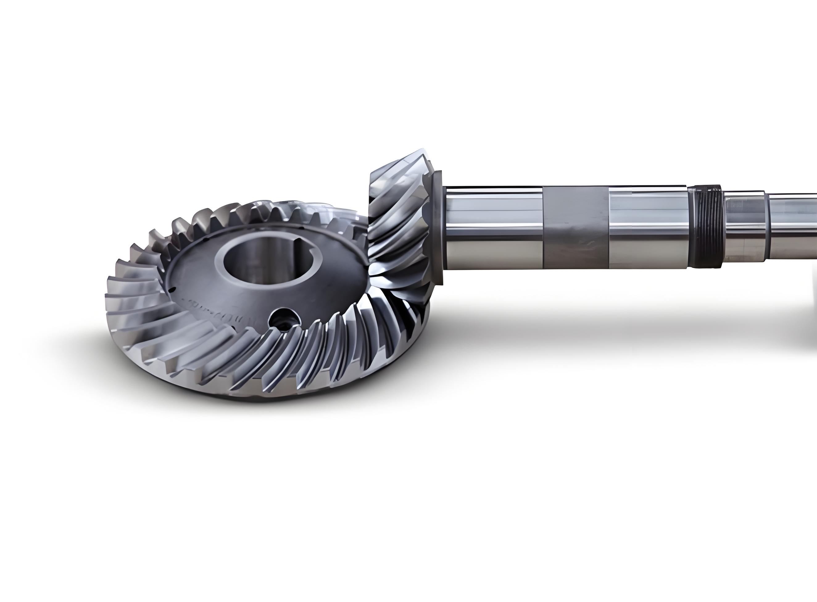
The following image shows a representative spiral bevel gear that helps me visualize the overall geometry before I proceed to the mathematical derivation.
I begin with the spherical involute. In the transmission motion of a spiral bevel gear, any point on the tooth surface remains at a fixed distance from the pitch cone apex, so the curve that forms the tooth surface can be treated as a spherical involute. When the rolling plane is tangent to the root cone along a cone generator and rolls without sliding on the cone surface, the trajectory of a fixed point on the rolling plane is the spherical involute. In a moving coordinate system \(O X’Y’Z’\), I write the vector \(OB\) as
$$ \begin{aligned} x’ &= l\sin\psi,\\ y’ &= 0,\\ z’ &= l\cos\psi, \end{aligned} $$
where \(l\) is the length of \(OB\), and
$$ \psi = \beta\sin\delta_f, $$
with \(\delta_f\) being the root cone angle. According to coordinate transformation theory, I can obtain coordinates at different positions on the tooth surface by changing \(\beta\) and \(l\). The moving coordinate system \(O X’Y’Z’\) and the fixed coordinate system \(O XYZ\) are related by the matrix expression
$$ \begin{bmatrix} x’\\ y’\\ z’ \end{bmatrix} = \begin{bmatrix} \sin\beta & -\cos\beta & 0\\ \cos\delta_f\cos\beta & \cos\delta_f\sin\beta & -\sin\delta_f\\ \sin\delta_f\cos\beta & \sin\delta_f\sin\beta & \cos\delta_f \end{bmatrix} \begin{bmatrix} x\\ y\\ z \end{bmatrix}. $$
Combining the moving-coordinate expression with the transformation matrix, I obtain the mathematical expression of the spherical involute as
$$ \begin{aligned} x &= l\left(\sin\beta\sin\psi + \cos\beta\cos\psi\sin\delta_f\right),\\ y &= l\left(\sin\beta\cos\psi\sin\delta_f – \cos\beta\sin\psi\right),\\ z &= l\cos\psi\cos\delta_f. \end{aligned} $$
For a spiral bevel gear, the distribution of the starting points of the spherical involute on the root cone determines the final tooth form. If the set of starting points follows a spiral line, the resulting gear is a spiral bevel gear. To preserve the cutting characteristics of a real spiral bevel gear, I introduce a spiral line based on the cutting principle. I consider a cutter disk at \(O_1\). The blade rotates with angular velocity \(\omega_1\), while the blade also revolves with angular velocity \(\omega\). To make the resultant motion of any point on the cutter disk a straight line along the \(X\) axis, I require
$$ \omega_1 = 2\omega. $$
For a point \(A\) on the cutter disk, the trajectory is then a straight line along the \(X\) axis, and its path equation is
$$ \begin{aligned} x &= -2r\sin(\omega t),\\ y &= 0,\\ z &= 0, \end{aligned} $$
where \(r\) is the cutter radius. I set the face-width coefficient to \(l/3\), and I use the cutter radius relation
$$ r = \frac{5}{6}R_x, $$
where \(R_x\) is the outer cone distance. The gear blank rotates with angular velocity \(\omega_2\). Since the root cone and the rolling plane are in pure rolling contact, the linear velocity at the common tangent point is the same, so I obtain
$$ \frac{\omega}{\omega_2} = \sin\delta_f. $$
The straight-line trajectory of point \(A\) is thus imprinted on the base cone surface as a conical spiral line. This is the key step that converts the spherical involute tooth profile into a spiral bevel gear tooth surface.
For my numerical example, I use a matched pair of spiral bevel gears. The large gear has \(43\) teeth, and the small gear has \(11\) teeth. The large-end module is \(m_s = 4.65\ \text{mm}\), the pressure angle is \(\alpha = 20^\circ\), the mean spiral angle is \(\beta_m = 30^\circ\), the shaft angle is \(\Sigma = 90^\circ\), the addendum coefficient is \(f = 0.85\), and the clearance coefficient is \(c = 0.188\). The basic parameters of the spiral bevel gear pair are summarized in Table 1.
| Parameter | Large spiral bevel gear | Small spiral bevel gear |
|---|---|---|
| Number of teeth \(z\) | 43 | 11 |
| Large-end module \(m_s\) (mm) | 4.65 | 4.65 |
| Pressure angle \(\alpha\) (deg) | 20 | 20 |
| Mean spiral angle \(\beta_m\) (deg) | 30 | 30 |
| Shaft angle \(\Sigma\) (deg) | 90 | 90 |
| Addendum coefficient \(f\) | 0.85 | 0.85 |
| Clearance coefficient \(c\) | 0.188 | 0.188 |
After calculation, I find that the two gears share several common geometric parameters. The outer cone distance is \(R_x = 103.1945\ \text{mm}\), the circular pitch is \(t = 14.6084\ \text{mm}\), the large-end addendum is \(h’ = 3.9525\ \text{mm}\), the large-end dedendum is \(h” = 4.8267\ \text{mm}\), the full tooth height is \(h = 8.7792\ \text{mm}\), the clearance is \(c_n = 0.8742\ \text{mm}\), the face width is \(b = 34.3981\ \text{mm}\), and the theoretical arc tooth thickness is \(s = 7.3042\ \text{mm}\). These common parameters are listed in Table 2.
| Common parameter | Symbol | Value |
|---|---|---|
| Outer cone distance | \(R_x\) | 103.1945 mm |
| Circular pitch | \(t\) | 14.6084 mm |
| Large-end addendum | \(h’\) | 3.9525 mm |
| Large-end dedendum | \(h”\) | 4.8267 mm |
| Full tooth height | \(h\) | 8.7792 mm |
| Clearance | \(c_n\) | 0.8742 mm |
| Face width | \(b\) | 34.3981 mm |
| Theoretical arc tooth thickness | \(s\) | 7.3042 mm |
I also calculate the individual parameters for the large and small spiral bevel gears. The pitch diameter is
$$ d = m_s z. $$
For a shaft angle of \(90^\circ\), the pitch cone angle is
$$ \delta = \arctan\left(\frac{z_1}{z_2}\right), $$
where \(z_1\) and \(z_2\) are the tooth numbers of the two mating gears. The outer cone distance can be written as
$$ R_x = \frac{d}{2\sin\delta}. $$
The individual calculated parameters are presented in Table 3.
| Parameter | Large spiral bevel gear | Small spiral bevel gear |
|---|---|---|
| Pitch diameter \(d\) (mm) | 199.95 | 51.15 |
| Pitch cone angle \(\delta\) (deg) | 75.6507 | 14.3493 |
| Root cone angle \(\delta_f\) (deg) | 72.9727 | 11.6714 |
| Base cone angle \(\delta_b\) (deg) | 62.3856 | 13.4655 |
| Addendum cone angle \(\delta_a\) (deg) | 77.8441 | 16.5428 |
I note that the calculated root cone angle of the small spiral bevel gear is smaller than its base cone angle. For a tapered-tooth spiral bevel gear, the root cone angle must be at least as large as the base cone angle. Therefore, I set the root cone angle of the small spiral bevel gear to \(13.4655^\circ\). This adjustment is important because it keeps the tooth surface generation consistent with the geometric constraints of the spiral bevel gear.
To generate the tooth-surface discrete points, I use MATLAB 2023a. I write a script that computes the concave and convex tooth surfaces of the large and small spiral bevel gears. The computational core is based on the following matrices:
$$ A = \begin{bmatrix} \cos\omega_2 & \sin\omega_2 & 0\\ -\sin\omega_2 & \cos\omega_2 & 0\\ 0 & 0 & 1 \end{bmatrix}, $$
$$ B = \begin{bmatrix} \sin\beta & -\cos\beta & 0\\ \cos\delta_f\cos\beta & \cos\delta_f\sin\beta & -\sin\delta_f\\ \sin\delta_f\cos\beta & \sin\delta_f\sin\beta & \cos\delta_f \end{bmatrix}, $$
$$ D = \begin{bmatrix} q\sin\psi\\ 0\\ q\cos\psi \end{bmatrix}. $$
The final coordinate vector is obtained from
$$ C = A B^{-1} D. $$
In my script, I discretize the motion parameters. For the small spiral bevel gear concave surface, I use a parameter \(j\) that ranges from \(0.6395\) to \(1\) with \(20\) intervals, and a parameter \(i\) that ranges from \(0\) to \(1\) with \(20\) intervals. I compute
$$ q = 2r\sin(\omega j), $$
$$ \omega_2 = \frac{\omega}{\sin\delta_f} j, $$
$$ \beta = \omega_1 i, $$
$$ \psi = \beta\sin\delta_f. $$
For each pair \((i,j)\), I calculate \(A\), \(B\), \(D\), and \(C\), and then I store the resulting \(x\), \(y\), and \(z\) coordinates. The convex-surface program is similar to the concave-surface program. For the large spiral bevel gear, I modify the root cone angle accordingly. The convex and concave surfaces of the same tooth have an angular offset at the starting point on the root cone. After simplifying the theoretical arc tooth thickness relation, I use an angular offset of
$$ \Delta\theta = \frac{\pi}{z}. $$
Because the two surfaces of one tooth move in opposite directions during pure rolling, I reverse the angle direction for the convex surface by adding a negative sign to the rotation angle in the transformation. This produces the correct orientation for the spiral bevel gear tooth surfaces. I save the large concave, large convex, small concave, and small convex point sets into four separate text files. The discrete-point generation parameters are summarized in Table 4.
| Generation item | Value or range |
|---|---|
| Software | MATLAB 2023a |
| Parameter \(j\) start | 0.6395 |
| Parameter \(j\) end | 1 |
| Parameter \(j\) intervals | 20 |
| Parameter \(i\) start | 0 |
| Parameter \(i\) end | 1 |
| Parameter \(i\) intervals | 20 |
| Output files | Large concave, large convex, small concave, small convex |
| File format | Text point cloud |
I then import the four discrete point files into UG NX 12.0. The modeling process for the spiral bevel gear pair follows a repeated sequence of surface fitting, sheet creation, trimming, blank creation, stitching, mirroring, arraying, and merging. First, I create a model file for the large spiral bevel gear and import the large concave and large convex point sets. I use the surface fitting command to fit smooth surfaces to the two point clouds. I repeat this process for the small spiral bevel gear in a separate model file.
Second, I draw the first tooth surface sheet. I sketch on the \(XZ\) plane using the cone distance, pitch cone angle, large-end dedendum, large-end addendum, and face width. I rotate the sketch sheet about the \(Z\) axis. I then extend both the fitted surface and the rotated sheet so that the four edges of the surface clearly exceed the rotated sheet. Using the trim sheet command, I remove the excess material and obtain the trimmed tooth-surface sheet. This operation is essential because the discrete points only define the tooth surface; the boundaries must be trimmed by the cone geometry of the spiral bevel gear.
Third, I draw the gear blank. On the \(XY\) plane, I sketch the blank rotation profile. I use two vertical dimensions related to the module: one value is \(4.65 \times 1.5\ \text{mm}\), and another value is \(4.65 \times 3\ \text{mm}\). I constrain these two lines to be perpendicular to the pitch generatrix. I extend the ends of the two lines horizontally to the gear blank axis, draw a line parallel to the gear blank axis, and trim the extra lines. I then rotate the sketch into a solid body. The resulting body is the gear blank for the large spiral bevel gear.
Fourth, I stitch the tooth-surface sheet and the gear blank into one body. I mirror the tooth-surface sheet about the \(XZ\) plane so that the hand of the large spiral bevel gear changes from left-hand to right-hand. I hide the original sheet, array the mirrored tooth surface \(43\) times, and merge the array result with the gear blank. This produces the complete large spiral bevel gear model. The modeling operations are summarized in Table 5.
| Modeling stage | Operation | Purpose |
|---|---|---|
| Point import | Import text point clouds | Bring discrete tooth-surface coordinates into the CAD environment |
| Surface fitting | Fit surface to points | Create smooth concave and convex surfaces |
| Sketching | Sketch on \(XZ\) plane | Define cone distance, cone angle, addendum, dedendum, and face width |
| Sheet rotation | Rotate sheet about \(Z\) axis | Create a conical cutting boundary |
| Extension and trim | Extend and trim sheets | Obtain bounded tooth-surface sheets |
| Blank creation | Sketch and rotate solid profile | Build the gear blank |
| Stitching | Stitch sheet and blank | Join the tooth surface to the blank |
| Mirroring | Mirror about \(XZ\) plane | Set the spiral bevel gear hand |
| Arraying | Array geometric feature | Create all teeth around the axis |
| Merging | Boolean merge | Form the final spiral bevel gear solid |
The small spiral bevel gear is modeled in a similar way. The main difference is that the pitch cone angle is \(14.3493^\circ\). Because the mating large and small spiral bevel gears have opposite hands, the small spiral bevel gear tooth surface does not need the same mirror operation. I array the small tooth surface \(11\) times and merge it with the small gear blank. To prepare for assembly, I add reference planes. For the large spiral bevel gear, I add a plane parallel to the \(XY\) plane at a distance of
$$ \frac{199.95}{2\tan 75.6507^\circ} = 25.5750\ \text{mm}, $$
and then I add a second parallel reference plane at a further distance of \(25.5750\ \text{mm}\). For the small spiral bevel gear, I add a reference plane at a distance of
$$ \frac{51.15}{2\tan 14.3493^\circ} = 99.9750\ \text{mm}. $$
These reference planes are used later in the assembly and motion simulation. To make coordinate measurement easier, I also model the large concave, large convex, small concave, and small convex tooth surfaces as individual single-tooth models. This is important because the probe of a coordinate measuring machine can approach a single tooth surface from a vertical direction more easily than it can approach a complete spiral bevel gear tooth inside a full gear body.
After building the spiral bevel gear models, I assemble them in Creo Parametric 9.0. I create an assembly file, define two perpendicular axes, and constrain the large and small spiral bevel gear axes to those axes. I use pin constraints. The large spiral bevel gear reference plane is made coincident with the top assembly plane, and the small spiral bevel gear reference plane is made coincident with the front assembly plane. This gives the correct \(90^\circ\) shaft angle and the correct axial positions. The assembly constraints are listed in Table 6.
| Assembly item | Constraint or definition |
|---|---|
| Assembly software | Creo Parametric 9.0 |
| Large spiral bevel gear axis | Coincident with vertical assembly axis |
| Small spiral bevel gear axis | Coincident with horizontal assembly axis |
| Large gear reference plane | Coincident with top assembly plane |
| Small gear reference plane | Coincident with front assembly plane |
| Constraint type | Pin |
| Shaft angle | \(90^\circ\) |
I then use the mechanism analysis module to define a gear pair. In the gear pair definition dialog, I choose the bevel type. For the first gear, which is the large spiral bevel gear, I select the large gear axis. For the second gear, which is the small spiral bevel gear, I select the small gear axis. In the properties page, I choose a user-defined transmission ratio. I enter a diameter \(D_1 = 199.95\ \text{mm}\), a diameter \(D_2 = 51.15\ \text{mm}\), a pressure angle of \(20^\circ\), and a spiral angle of \(30^\circ\). I select a plane on the large spiral bevel gear as the icon position and accept the remaining defaults. After the gear pair is defined, I use the drag component command. When I drag a tooth of the small spiral bevel gear, the small gear rotates and the large spiral bevel gear rotates simultaneously. The motion is smooth and the assembly is successful.
For additive manufacturing, I export the completed spiral bevel gear models as STL files from UG NX 12.0. I slice the models in a slicing program. The key printing parameters are a layer height of \(0.2\ \text{mm}\), a wall thickness of \(1.2\ \text{mm}\), a bottom and top thickness of \(1.0\ \text{mm}\), an infill density of \(10\%\), a printing speed of \(40\ \text{mm/s}\), a nozzle temperature of \(210^\circ\text{C}\), and a heat bed temperature of \(40^\circ\text{C}\). I use local support, a brim for platform adhesion, PLA material with a diameter of \(1.75\ \text{mm}\), and an extrusion multiplier of \(100\%\). The printing settings are summarized in Table 7.
| Printing parameter | Value |
|---|---|
| Layer height | 0.2 mm |
| Wall thickness | 1.2 mm |
| Bottom and top thickness | 1.0 mm |
| Infill density | 10% |
| Printing speed | 40 mm/s |
| Nozzle temperature | 210 °C |
| Heat bed temperature | 40 °C |
| Support type | Local support |
| Platform adhesion | Brim |
| Material | PLA |
| Filament diameter | 1.75 mm |
| Extrusion multiplier | 100% |
I print the complete large and small spiral bevel gears. The large spiral bevel gear requires \(18.5\ \text{h}\), \(63.89\ \text{m}\) of filament, and \(191\ \text{g}\) of material. The small spiral bevel gear requires \(2.7\ \text{h}\), \(8.51\ \text{m}\) of filament, and \(25\ \text{g}\) of material. These values are shown in Table 8. The printed large and small spiral bevel gears mesh smoothly, which provides a practical verification that the modeled tooth surfaces are geometrically compatible.
| Spiral bevel gear component | Print time (h) | Filament length (m) | Material weight (g) |
|---|---|---|---|
| Large spiral bevel gear | 18.5 | 63.89 | 191 |
| Small spiral bevel gear | 2.7 | 8.51 | 25 |
I also print the four single-tooth surface models separately. The large concave surface requires \(7.13\ \text{h}\), \(15.43\ \text{m}\), and \(46\ \text{g}\). The large convex surface requires \(15.24\ \text{h}\), \(33.29\ \text{m}\), and \(99\ \text{g}\). The small concave surface requires \(6.77\ \text{h}\), \(14.78\ \text{m}\), and \(44\ \text{g}\). The small convex surface requires \(7\ \text{h}\), \(15.55\ \text{m}\), and \(46\ \text{g}\). These results are listed in Table 9.
| Single tooth surface | Print time (h) | Filament length (m) | Material weight (g) |
|---|---|---|---|
| Large concave | 7.13 | 15.43 | 46 |
| Large convex | 15.24 | 33.29 | 99 |
| Small concave | 6.77 | 14.78 | 44 |
| Small convex | 7 | 15.55 | 46 |
To inspect the tooth surfaces, I create measurement point sets on the large and small spiral bevel gear concave and convex surfaces in UG. I use a \(U\)-\(V\) grid. For the large concave, large convex, small concave, and small convex surfaces, I use \(12\) points in the \(U\) direction and \(8\) points in the \(V\) direction, giving \(96\) points per surface. The start and end percentages differ slightly for the small gear because of the available surface area and the need to avoid edge effects. The measurement point plan is summarized in Table 10.
| Surface | Large concave | Large convex | Small concave | Small convex |
|---|---|---|---|---|
| \(U\) count | 12 | 12 | 12 | 12 |
| \(V\) count | 8 | 8 | 8 | 8 |
| Start \(U\) (%) | 10 | 10 | 10 | 10 |
| End \(U\) (%) | 90 | 90 | 80 | 85 |
| Start \(V\) (%) | 25 | 25 | 28 | 25 |
| End \(V\) (%) | 75 | 75 | 60 | 65 |
| Total points per surface | 96 | 96 | 96 | 96 |
I extract the point sets from the spiral bevel gear tooth surfaces and convert them into text files. I then use an improved ant colony algorithm to plan the measurement path. The purpose of path planning is to order the measurement points so that the coordinate measuring machine can inspect them automatically and efficiently. Without planning, each of the \(96\) points on a surface would need to be selected manually, which takes much longer. The inspection equipment is a Hexagon Leitz Reference HP coordinate measuring machine with PC-DMIS software. The maximum permissible error is \(MPE_E = 0.9 + L/400\ \mu\text{m}\). The probe sphere diameter is \(5\ \text{mm}\), the positioning and retraction distance is \(3\ \text{mm}\), the moving speed is \(20\ \text{mm/s}\), and the touch and retraction speed is \(2\ \text{mm/s}\).
During measurement, I clamp the single-tooth surface model, establish the measurement coordinate system by best fitting, import the planned path, and let the probe perform automatic inspection. The planned path reduces the inspection time. For the large concave surface, the unplanned inspection time is \(637\ \text{s}\), while the planned inspection time is \(467\ \text{s}\), a reduction of \(26.65\%\). For the large convex surface, the times are \(646\ \text{s}\) and \(476\ \text{s}\), a reduction of \(26.35\%\). For the small concave surface, the times are \(627\ \text{s}\) and \(457\ \text{s}\), a reduction of \(27.13\%\). For the small convex surface, the times are \(630\ \text{s}\) and \(466\ \text{s}\), a reduction of \(26.03\%\). These results are given in Table 11.
| Surface | Unplanned inspection time (s) | Planned inspection time (s) | Reduction (%) |
|---|---|---|---|
| Large concave | 637 | 467 | 26.65 |
| Large convex | 646 | 476 | 26.35 |
| Small concave | 627 | 457 | 27.13 |
| Small convex | 630 | 466 | 26.03 |
After inspection, I analyze the measured data. For each measured point, I compute the deviation between the measured point and the nominal point. I use the signed normal error
$$ e_i = \mathbf{n}_i \cdot \left(\mathbf{p}_i^{\text{meas}} – \mathbf{p}_i^{\text{nom}}\right), $$
where \(\mathbf{n}_i\) is the unit normal at the nominal point, \(\mathbf{p}_i^{\text{meas}}\) is the measured point, and \(\mathbf{p}_i^{\text{nom}}\) is the nominal point. I also compute the mean error, root-mean-square error, and standard deviation as
$$ \bar e = \frac{1}{N}\sum_{i=1}^{N} e_i, $$
$$ RMS = \sqrt{\frac{1}{N}\sum_{i=1}^{N} e_i^2}, $$
$$ \sigma = \sqrt{\frac{1}{N-1}\sum_{i=1}^{N}\left(e_i-\bar e\right)^2}. $$
The measured results show that the large concave surface has a 3D printing error range of \(0\) to \(0.16\ \text{mm}\). The large convex surface has a 3D printing error range of \(0\) to \(0.06\ \text{mm}\). The small concave surface has a 3D printing error range of \(0\) to \(0.15\ \text{mm}\). The small convex surface has a 3D printing error range of \(0\) to \(0.15\ \text{mm}\). These error ranges are summarized in Table 12. The overall average error of the tooth surfaces is therefore in the range of \(0\) to \(0.16\ \text{mm}\), which verifies the effectiveness of the spherical-involute-based modeling method for the spiral bevel gear.
| Tooth surface | 3D printing error range (mm) |
|---|---|
| Large concave | 0 to 0.16 |
| Large convex | 0 to 0.06 |
| Small concave | 0 to 0.15 |
| Small convex | 0 to 0.15 |
| Overall average range | 0 to 0.16 |
The error distribution of the small concave surface is representative of the other surfaces. The histogram shows that most deviations are concentrated near the lower end of the error range, while a smaller number of points reach the upper end. This indicates that the nominal tooth surface is well defined and that the larger deviations are mainly caused by the 3D printing process rather than by the mathematical model. If I optimize the printing parameters, such as layer height, extrusion consistency, support removal, and thermal shrinkage compensation, I can further improve the 3D printing accuracy of the spiral bevel gear tooth surfaces.
I draw several conclusions from this work. First, the spherical involute theory provides a consistent basis for describing the tooth surface of a spiral bevel gear. By changing the generating parameters, I can obtain discrete points on both the concave and convex surfaces of a mating large and small spiral bevel gear pair. Second, the use of MATLAB to generate discrete point coordinates and UG NX to fit and trim surfaces makes the spiral bevel gear modeling process systematic and repeatable. Third, the assembly and motion simulation in Creo Parametric 9.0 confirm that the modeled large and small spiral bevel gears mesh correctly and rotate together with the expected transmission ratio. Fourth, the 3D printed spiral bevel gear pair exhibits smooth meshing, which provides physical evidence that the model is geometrically valid. Fifth, the coordinate measuring machine inspection and path planning show that the tooth surface error can be measured automatically and efficiently. The planned path reduces inspection time by more than \(26\%\) in all four cases.
For future work, I would optimize the 3D printing parameters to reduce the average tooth-surface error of the spiral bevel gear. I would also extend the method to other tooth numbers, modules, spiral angles, and shaft angles so that the same spherical-involute-based workflow can be used for a wider family of spiral bevel gear pairs. I would further investigate how the discrete point density affects surface fitting quality, because a higher point density may improve geometric fidelity but also increase computation and measurement time. Finally, I would compare the measured tooth surface with the nominal surface using more advanced registration and compensation algorithms, so that the spiral bevel gear model can be corrected for manufacturing and printing deviations.
In summary, my first-person workflow for the spiral bevel gear starts from spherical involute geometry, proceeds through discrete point generation, CAD surface fitting, solid modeling, assembly, motion simulation, 3D printing, measurement point planning, and coordinate inspection, and ends with quantitative error analysis. The results confirm that a spiral bevel gear can be modeled accurately and efficiently by combining analytical derivation with numerical computation and experimental verification. The average tooth-surface error of \(0\) to \(0.16\ \text{mm}\) and the smooth meshing of the printed pair support the validity of the method. This gives me confidence that the same approach can be applied to more complex spiral bevel gear design, manufacturing, and inspection tasks.