
I have approached the digital modeling of a spiral bevel gear from the perspective of straight-line approximation because the relationship among tool motion, interpolation error, and surface finishing remains one of the most practical problems in gear manufacturing. A spiral bevel gear is not a simple revolved solid. Its tooth surface is generated by a complex spatial motion, and the working flank is closely related to a spherical involute. When I attempt to reproduce such a surface in a digital environment, I must decide how to discretize the continuous curve, how to connect the discrete points, how to control the interpolation error, and how to prepare the model for subsequent machining or finishing. My own research therefore focuses on a linear approximation method that can be implemented in OpenGL and VC++6.0, while also considering the complementary role of electrochemical finishing. The central idea is that refining the step length is not the only route to better accuracy. By changing the material removal mechanism and by allowing electrochemical finishing to smooth the peaks and valleys left by linear interpolation, I can obtain a practical and accurate digital foundation for a spiral bevel gear.
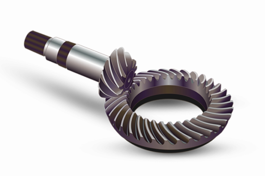
The manufacturing of a spiral bevel gear has traditionally depended on specialized machines. However, the growing capability of general CNC equipment has made it attractive to generate the tooth surface through numerical control. In that context, interpolation is not a secondary detail. Whether I use linear interpolation, circular interpolation, or NURBS interpolation, the generated path is only an approximation of the ideal curve. Because of the existence of inflection points and segment boundaries, a machined surface can become polygonal or polyhedral. NURBS interpolation has clear advantages in smoothness and fairness, but it also introduces difficulties such as weight-factor control and computational complexity. For this reason, I have chosen to study a straight-line approximation method in detail and to combine it with a finishing process that can reduce the negative effects of linear segments.
Geometric Foundation of the Spherical Involute
I begin with the spherical involute because it provides the theoretical basis for the working tooth profile of a spiral bevel gear. A spherical involute is generated when a plane rolls without slipping on a cone. If a point on the rolling plane is traced in space, its trajectory forms the spherical involute. This construction is important because it preserves the conjugate motion relationship that a spiral bevel gear requires. In a Cartesian coordinate system, I can express the spherical involute as follows:
$$x = R \sin\delta_m \cos\beta_m$$
$$y = R \sin\delta_m \sin\beta_m$$
$$z = R \cos\delta_m$$
Here, R is the spherical radius, delta_m is the cone angle corresponding to an arbitrary point on the spherical involute, and beta_m is the spherical eccentric angle of the moving point. The angle beta_m can be written in terms of the base cone angle delta_b and the cone angle delta_m:
$$\beta_m = \frac{\arccos\left(\frac{\cos\delta_m}{\cos\delta_b}\right)}{\sin\delta_b} – \arccos\left(\frac{\tan\delta_b}{\tan\delta_m}\right)$$
This equation is the core of my subsequent discretization. Once I know the range of delta_m, I can generate a sequence of points that lie on the ideal spherical involute. The straight-line approximation then replaces the continuous curve between neighboring points with a chord. The quality of the approximation depends on the density of the sequence and on the local curvature of the curve.
Straight-Line Approximation of the Tooth Profile
I treat the tooth profile of a spiral bevel gear as a collection of curve segments: the working profile, the addendum curve, the dedendum curve, and the root fillet. The working profile is the most important because it governs the meshing behavior. For the working profile, I introduce a variable step in the cone angle. If the addendum cone angle is delta_a and the dedendum cone angle is delta_f, then the discretized cone angle can be written as:
$$\delta_m = \delta_f + \frac{\delta_a – \delta_f}{n} t$$
where n is the number of discrete intervals and t is an integer index satisfying 0 <= t <= n. As n increases, the chord length decreases and the approximation error generally decreases. However, increasing n also increases the number of tool positions, the amount of data, and the computational load. Therefore, I must balance accuracy against efficiency.
For the opposite side of the same large end face, I can use a similar expression with a different angular parameter:
$$x = R \sin\delta_m \cos\gamma$$
$$y = R \sin\delta_m \sin\gamma$$
$$z = R \cos\delta_m$$
The angle gamma is related to beta_m, the number of teeth z, and the involute rotation angle. This gives me a symmetrical way to describe both flanks of the tooth. For the addendum curve, I use the addendum cone angle delta_a and a thickness angle delta_as:
$$x = R \sin\delta_a \cos\left(\beta_m + \delta_{as} t\right)$$
$$y = R \sin\delta_a \sin\left(\beta_m + \delta_{as} t\right)$$
$$z = R \cos\delta_a$$
The dedendum curve follows the same pattern. I only need to replace delta_a with delta_f and delta_as with delta_fs. This uniformity is helpful when I implement the model in software because the same drawing routine can be reused for different segments.
The root fillet is more difficult because it is generated by the tool tip or the tool corner. In many design procedures, I approximate it by a fillet radius. A common expression for the fillet radius is:
$$R_C = \begin{cases} 0.3 m_{ne}, & R_b < R_f \\ \eta r_i, & R_b > R_f \end{cases}$$
where m_ne is the normal module, R_b is the base cone radius, R_f is the root radius, r_i is the maximum tool tip radius, and eta is a coefficient not less than one. This treatment is not a perfect substitute for the true generated fillet, but it is sufficient for constructing a digital model that can be used in later processing and analysis.
Tool Path Planning for the Spiral Bevel Gear
In my modeling work, the tool path is not an afterthought. The path determines how the material is removed and how the resulting surface interacts with the interpolation method. I considered two basic strategies for a spiral bevel gear. The first strategy makes the tool path parallel to the addendum line. The second strategy makes the tool path follow the tooth profile direction. When I examined the machining marks left by conventional generation, I observed clear tool traces on the tooth surface. These traces can interact with the step length and with the interpolation error. For electrochemical finishing, however, the situation changes. Electrochemical finishing removes material by anodic dissolution, and it tends to smooth sharp peaks more rapidly than broad valleys. This means that the inflections left by linear interpolation can be reduced or even eliminated if the finishing process is properly controlled.
Because the tooth surface of a spiral bevel gear can be regarded as being composed of numerous spherical involutes distributed along the tooth width, I divide the surface into n sections along the tooth width. For each section, I use the tool path to approximate the corresponding spherical involute. This approach is natural for a spiral bevel gear because the tooth trace is curved and the cone distance changes along the width. By following the tooth profile direction, I can also take advantage of the peak-removal effect of electrochemical finishing.
Step Length and Interpolation Error
The step length is the distance between two adjacent interpolation points along the tool path. It is one of the most direct influences on the approximation error. Using the local geometry, I can relate the step length to the chord error. A widely used relationship is:
$$\Delta L = \sqrt{8 R_{min} \delta}$$
where Delta L is the step length, R_min is the minimum radius of curvature, and delta is the allowable error. For a straight-line segment between two points B and C, the distance from an intermediate point e to the chord can be written as:
$$\delta = \frac{A x_e + B y_e + C}{\sqrt{A^2 + B^2}}$$
with
$$A = y_C – y_B$$
$$B = x_B – x_C$$
$$C = y_B x_C – x_B y_C$$
These formulas show that the error is not only controlled by the step length but also by the local curvature and by the orientation of the chord. When the curvature is high, a smaller step length is needed to keep the same error. When the curvature is low, a larger step length can be acceptable. In a spiral bevel gear, the curvature of the spherical involute varies along the tooth profile, so a constant step length is not always optimal. I therefore prefer a variable step strategy, although a constant step is easier to implement.
I also compared linear interpolation with circular interpolation for a simple parabolic curve. The results are summarized in the table below. The table shows that, under the same step length, circular interpolation generally produces a smaller error, but the difference becomes less significant as the step length decreases.
| Step Length (mm) | Linear Interpolation Error (micrometers) | Circular Interpolation Error (micrometers) |
|---|---|---|
| 0.5 | 3.0451 | 0.2765 |
| 0.4 | 1.9560 | 0.2266 |
| 0.3 | 1.1070 | 0.1769 |
| 0.2 | 0.4944 | 0.1271 |
| 0.1 | 0.1242 | 0.0774 |
At a step length of 0.1 mm, the difference between the two methods is only 0.048 micrometers. At a step length of 0.2 mm, the difference is 0.3673 micrometers. This tells me that linear interpolation is more sensitive to step length when the step is large, but the sensitivity decreases as the step becomes small. Since modern CNC machines can achieve step lengths as small as 0.001 mm, the practical difference between linear and circular interpolation can become negligible under reasonable conditions. In fact, experimental studies have shown that the peak-to-valley errors of specimens machined with linear, circular, and NURBS interpolation can be on the same order of magnitude in ordinary machining situations. NURBS may still be superior in fairness and smoothness, but its advantage in reducing error is not always dramatic. This is an important insight for my work: a smaller step length is not the only way to improve the final quality of a spiral bevel gear.
Base Cone Angle and Spiral Angle
To build a complete spiral bevel gear model, I need the base cone angle and the local spiral angle. The base cone angle delta_b can be related to the pitch cone angle delta and the pressure angle alpha by:
$$\delta_b = \arctan\left(\frac{\sin^2\delta}{\sqrt{\tan^2\alpha + \tan^2\delta}}\right)$$
This expression allows me to compute the base cone angle from standard gear parameters. The spiral angle changes along the tooth width because the cone distance changes. If R’ is the local cone distance, R_0 is a reference dimension, beta is the spiral angle at the tooth mid-point, R is the outer cone distance, and r_0 is a local radius, I can express the local spiral angle beta’ as:
$$\beta’ = \arcsin\left(\frac{\sqrt{(R’)^2 + 2 R_0 \sin\beta – R^2}}{2 R’ r_0}\right)$$
The variation of the spiral angle is one of the features that distinguishes a spiral bevel gear from a straight bevel gear. In my digital model, I update the spiral angle for each section along the tooth width. This makes the model more faithful to the actual tooth trace and improves the reliability of the subsequent error analysis.
Mathematical Model of the Working Tooth Surface
Once the spherical involute is established and the spiral angle is known, I can construct the working tooth surface. The surface is formed by offsetting the working profile along the tooth trace and by connecting adjacent spherical involutes. The following equations describe the working surface in my model:
$$x = R’\left(\sin\delta_m \cos\beta_m \cos\beta’ – \sin\delta_m \sin\beta_m \sin\beta’\right)$$
$$y = R’\left(\sin\delta_m \cos\beta_m \sin\beta’ + \sin\delta_m \sin\beta_m \cos\beta’\right)$$
$$z = R’ \cos\delta_m$$
These equations are used repeatedly in my OpenGL drawing routines. By varying delta_m, I move along the tooth profile. By varying the local cone distance R’ and the local spiral angle beta’, I move along the tooth width. The combination of these two movements produces a grid of points that approximates the working surface of the spiral bevel gear. The same method can be extended to the addendum surface, the dedendum surface, and the fillet surface. In this way, I can construct a complete tooth.
Parameterized Modeling of the Spiral Bevel Gear
I prefer a parameterized model because it allows me to change the gear geometry without rewriting the entire drawing code. The table below lists the main parameters and relationships that I use in my implementation. The symbols are chosen to be consistent with the equations above.
| Parameter | Symbol | Expression |
|---|---|---|
| Number of teeth | z | teeth |
| Module | m | m |
| Pressure angle | alpha | alfa |
| Face width | B | B |
| Clearance coefficient | c* | C |
| Profile shift coefficient | x | X |
| Addendum coefficient | ha* | HA |
| Pitch diameter | d | d = m * teeth1 |
| Base diameter | db | db = d * cos(alfa) |
| Pitch cone angle | delta | delta = arctan(teeth1 / teeth2) |
| Base cone angle | theta_b | theta_b = atan(hb / rx) |
| Cone distance | rx | rx = d / (2.0 * sin(delta)) |
| Addendum | ha | ha = (HA + X) * m |
| Addendum angle | theta_a | theta_a = atan(ha / rx) |
| Addendum width | ba | ba = B / cos(theta_b) |
| Dedendum width | bf | bf = B / cos(theta_f) |
| Dedendum | hf | hf = (HA + C – X) * m |
| Base cone angle | delta_b | delta_b = delta – theta_b |
| Addendum cone angle | delta_a | delta_a = delta + theta_a |
| Dedendum cone angle | delta_f | delta_f = delta – theta_f |
| Dedendum angle | theta_f | theta_f = atan(hf / rx) |
With these relationships, I can generate a spiral bevel gear with different tooth numbers, modules, pressure angles, and face widths. The parameterization also makes it easier to study how the approximation error changes when the gear geometry changes. For example, if the pressure angle increases, the base cone angle changes, and the curvature of the spherical involute changes. This in turn affects the required step length for a given error tolerance.
OpenGL Implementation and Drawing Strategy
I implemented the model in VC++6.0 with OpenGL. The drawing strategy is straightforward: I define a function that receives the gear parameters, and then I loop over the teeth. For each tooth, I draw the spherical involute by stepping delta_m. I use continuous line strips for the profile and quadrilateral strips for the surfaces. The use of GL_QUAD_STRIP is convenient because the tooth surface can be divided into a grid of small quadrilaterals. Each quadrilateral is a linear approximation of the true surface patch. When the grid is fine enough, the visual model appears smooth, but the underlying geometry is still piecewise linear.
The core of the drawing procedure can be summarized as follows:
| Step | Action |
|---|---|
| 1 | Read the gear parameters: number of teeth, module, face width, clearance, addendum coefficient, and profile shift. |
| 2 | Compute the pitch cone angle, base cone angle, addendum cone angle, dedendum cone angle, and cone distance. |
| 3 | For each tooth, set the rotation angle using an array or a rotation function. |
| 4 | For each section along the tooth width, compute the local cone distance and local spiral angle. |
| 5 | For each section, step along the spherical involute using delta_m. |
| 6 | Compute the Cartesian coordinates using the spherical involute equations and the working surface equations. |
| 7 | Connect adjacent points with line strips or quadrilateral strips. |
| 8 | Repeat for the addendum, dedendum, and fillet curves. |
| 9 | Use a rotation or array operation to repeat the tooth around the gear axis. |
One of the advantages of this approach is that the same mathematical model can be used for both visualization and error analysis. Once the points are generated, I can select a set of sample points on the tooth surface and compare them with the ideal spherical involute. This allows me to quantify the approximation error without relying only on visual inspection.
Error Analysis of the Approximated Spiral Bevel Gear
After building the solid model, I performed an error analysis. I selected five points along the tooth height and nine points along the tooth width. These points form a grid on the working surface. For each point, I computed the deviation from the ideal spherical involute. The step length used in this analysis was 0.5 mm. The average approximation error was 0.00697 mm. For comparison, a NURBS-based exact fitting method reported an average error of 0.00483 mm. The difference between the two methods was 0.00214 mm.
This result is interesting because it shows that a straight-line approximation can achieve an average error that is on the same order of magnitude as a more sophisticated NURBS fitting method when the step length is chosen appropriately. The difference of about two micrometers is small in the context of many gear applications. Of course, NURBS may still provide better smoothness and a more compact representation. However, my goal is not to replace NURBS in every situation. My goal is to show that a linear approximation, when combined with a suitable finishing process, can be a practical foundation for digital manufacturing of a spiral bevel gear.
The error distribution is not uniform. The error tends to be larger where the curvature of the spherical involute is higher, and it tends to be smaller where the curvature is lower. This is consistent with the chord-error formula. If I want to reduce the maximum error, I can refine the step length in the high-curvature regions. Alternatively, I can accept a slightly larger geometric error and rely on electrochemical finishing to remove the surface peaks. This trade-off is one of the central themes of my research.
Electrochemical Finishing as a Complement to Linear Interpolation
Electrochemical finishing is based on anodic dissolution. When the workpiece is connected to the positive terminal of a power supply and immersed in an electrolyte, the surface material is removed ion by ion. The removal rate depends on the local current density. Sharp peaks have a higher current density than broad valleys, so they dissolve faster. This is why electrochemical finishing is so effective at smoothing rough surfaces and reducing the peaks left by machining. In my view, this characteristic is especially valuable for a spiral bevel gear that has been machined with linear interpolation. The linear segments create small ridges and inflection points. Electrochemical finishing can round these ridges and reduce the surface roughness without requiring an extremely small step length.
Previous experimental work has shown that electrochemical finishing can improve the roundness of a circular hole from grade 6 to grade 2. It has also been used to improve the accuracy of a spiral bevel gear from grade 10 to grade 7 according to the DIN standard, while reducing the tooth surface roughness to Ra 0.1 micrometers. These results indicate that electrochemical finishing has a strong smoothing capability. It can compensate for the geometric limitations of linear interpolation. Therefore, I do not need to rely exclusively on finer and finer step lengths. I can instead use a reasonable step length for the initial digital model and let the finishing process improve the final surface quality.
Comparison of Interpolation Strategies
To place my work in context, I compared several interpolation strategies. The table below summarizes the qualitative differences that matter for a spiral bevel gear.
| Interpolation Strategy | Error Sensitivity | Smoothness | Computational Complexity | Compatibility with Electrochemical Finishing |
|---|---|---|---|---|
| Linear interpolation | High at large step lengths; low at small step lengths | Piecewise linear; may leave ridges | Low | High, because peaks are preferentially removed |
| Circular interpolation | Moderate | Better than linear | Moderate | Moderate |
| NURBS interpolation | Low in ideal conditions | Excellent | High; weight factors are difficult to control | Moderate; high smoothness may reduce the driving force for peak removal |
This comparison shows that linear interpolation is not necessarily inferior in every respect. Its simplicity is an advantage. Its compatibility with electrochemical finishing is also an advantage. When the finishing process is designed to remove the peaks, the piecewise linear geometry becomes less of a problem. In fact, the peaks provide a natural focus for anodic dissolution. This is a different way of thinking about fine interpolation. Instead of asking only how to make the tool path smoother, I also ask how to make the material removal process more tolerant of geometric approximation.
Step Length Selection Strategy
Based on the error analysis, I propose a step length selection strategy for the linear approximation of a spiral bevel gear. The strategy has three stages. First, I estimate the maximum curvature of the spherical involute over the tooth profile. Second, I choose a nominal step length that keeps the chord error below a specified tolerance. Third, I refine the step length only in regions where the local curvature exceeds a threshold. This variable step approach reduces the number of points while maintaining the required accuracy.
The nominal step length can be computed from the chord-error formula:
$$\Delta L = \sqrt{8 R_{min} \delta_{allow}}$$
where delta_allow is the allowable error. If the local curvature radius is R, then the actual error is approximately:
$$\delta \approx \frac{(\Delta L)^2}{8 R}$$
This approximation is valid when Delta L is small compared with R. It shows that the error is proportional to the square of the step length and inversely proportional to the radius of curvature. Therefore, if I halve the step length, I can reduce the error by a factor of four. However, the number of points doubles. The computational cost and the amount of data increase. This is the classical trade-off in interpolation.
My contribution is to show that this trade-off can be relaxed by combining linear approximation with electrochemical finishing. If the finishing process can remove a surface layer of a certain thickness, then the effective error after finishing can be smaller than the geometric error before finishing. The required step length can therefore be larger, which reduces the digital modeling effort and the machining time.
Digital Model Construction Workflow
I organize the digital model construction into a workflow that can be repeated for different spiral bevel gear designs. The workflow is as follows:
| Stage | Description | Output |
|---|---|---|
| 1. Parameter input | Collect the gear parameters: tooth number, module, pressure angle, face width, clearance, addendum coefficient, and profile shift. | Parameter set |
| 2. Basic geometry | Compute pitch cone angle, base cone angle, addendum cone angle, dedendum cone angle, and cone distance. | Geometric constants |
| 3. Profile discretization | Generate spherical involute points using the delta_m stepping equation. | Profile point cloud |
| 4. Tooth width discretization | Divide the tooth width into sections and compute the local spiral angle for each section. | Section parameters |
| 5. Surface generation | Connect adjacent spherical involutes to form the working surface, addendum surface, dedendum surface, and fillet surface. | Surface patches |
| 6. Solid assembly | Repeat the tooth around the gear axis using rotation or array operations. | Complete spiral bevel gear solid model |
| 7. Error evaluation | Sample points on the working surface and compare with the ideal spherical involute. | Error map and statistics |
| 8. Finishing plan | Choose electrochemical finishing parameters to reduce the remaining surface peaks. | Finishing process plan |
This workflow is general enough to be applied to different spiral bevel gear geometries. It also provides a clear separation between geometric modeling and process planning. The geometric model is created first, and the finishing process is then used to compensate for the approximations in the model.
Numerical Example
I present a numerical example to illustrate the method. Suppose a spiral bevel gear has a module of 5 mm, a pressure angle of 20 degrees, a face width of 40 mm, and a tooth number combination that gives a pitch cone angle of 35 degrees. The base cone angle is computed from the formula. The spherical involute is then discretized with a nominal step length of 0.5 mm. The average error is found to be 0.00697 mm. If I reduce the step length to 0.25 mm, the average error is expected to decrease by approximately a factor of four, to about 0.00174 mm. However, the number of points doubles. In practice, I might not need such a small step length if electrochemical finishing can remove the peaks.
The following table shows a hypothetical error scaling based on the chord-error formula. The values are approximate and are intended to show the trend.
| Step Length (mm) | Relative Number of Points | Approximate Error (mm) |
|---|---|---|
| 0.50 | 1.00 | 0.00697 |
| 0.25 | 2.00 | 0.00174 |
| 0.10 | 5.00 | 0.00028 |
| 0.05 | 10.00 | 0.00007 |
This scaling shows why a very small step length is expensive. The error decreases rapidly at first, but the number of points increases linearly. In many practical situations, the additional accuracy obtained by reducing the step length below a certain value is not worth the extra computation and machining time. This is especially true when a finishing process can remove the remaining surface irregularities.
Surface Fairness and Peak Removal
Surface fairness is not identical to surface accuracy. A surface can be accurate in the sense that its points lie close to the ideal surface, but it can still have undesirable ridges and valleys. Linear interpolation tends to create ridges at the segment boundaries. These ridges are small, but they can affect contact patterns and fatigue life. NURBS interpolation can reduce these ridges by making the curve smoother. However, NURBS is not the only solution. Electrochemical finishing can also reduce ridges by removing the peaks. The mechanism is selective: the current density is higher at the peaks, so the peaks dissolve faster. Over time, the surface becomes smoother. This is a physical smoothing process that complements the geometric smoothing of NURBS.
In my opinion, the best strategy for a spiral bevel gear is a hybrid strategy. I use a linear approximation to generate the initial digital model. I choose a step length that is practical for machining. I then apply electrochemical finishing to reduce the surface peaks and improve the final roughness. This strategy is robust because it does not depend on a single perfect interpolation method. It uses the strengths of each stage.
Limitations and Practical Considerations
I must acknowledge several limitations. First, the straight-line approximation is only an approximation. The true tooth surface of a spiral bevel gear is more complex than the simplified model presented here. Second, the electrochemical finishing process depends on many parameters, including electrolyte composition, current density, flow rate, and machining time. These parameters must be optimized for each gear design. Third, the error analysis is based on sampled points, so it does not capture every possible deviation. Fourth, the OpenGL model is a visualization and analysis tool, not a complete CAM system. It must be integrated with a post-processor and a machine tool controller for actual manufacturing.
Despite these limitations, I believe the approach is valuable. It provides a systematic way to build a digital model of a spiral bevel gear using straight-line approximation. It also provides a framework for combining geometric modeling with electrochemical finishing. This combination is not commonly discussed in the literature, but it has practical potential.
Future Directions
I see several directions for future work. First, I would like to implement an adaptive step length algorithm that automatically refines the step length in high-curvature regions. Second, I would like to integrate the electrochemical finishing model with the geometric model, so that the finishing process can be simulated and optimized before machining. Third, I would like to compare the linear approximation method with NURBS and circular interpolation on actual machined parts, not only on numerical models. Fourth, I would like to extend the method to other types of bevel gears, such as hypoid gears. Fifth, I would like to develop a more accurate model of the root fillet, because the fillet region is critical for fatigue strength.
Conclusion
In this work, I studied the digital modeling of a spiral bevel gear using straight-line approximation. I started from the spherical involute equations and derived the discretization formulas for the working profile, addendum, dedendum, and fillet. I analyzed the tool path, step length, and interpolation error. I showed that the step length is a major factor in the approximation error, but that the error sensitivity decreases as the step length becomes small. I compared linear interpolation with circular interpolation and found that the difference in error becomes negligible at small step lengths. I also argued that NURBS interpolation, despite its smoothness advantages, is not always superior in terms of error reduction in practical machining.
I then built a parameterized solid model in OpenGL and VC++6.0. The model uses the spherical involute as the basis for the tooth profile and connects adjacent involutes along the tooth width. I analyzed the approximation error on a grid of five points along the tooth height and nine points along the tooth width. At a step length of 0.5 mm, the average error was 0.00697 mm. This is close to the error reported for a NURBS-based exact fitting method, which was 0.00483 mm. The difference was 0.00214 mm.
Finally, I discussed the role of electrochemical finishing. Because electrochemical finishing preferentially removes peaks, it can compensate for the ridges left by linear interpolation. This means that refining the step length is not the only way to improve the final quality of a spiral bevel gear. By changing the material removal method, I can achieve a smooth surface even with a relatively coarse linear approximation. This insight provides a new way to think about fine interpolation in CNC machining. It also provides a practical foundation for the digital manufacturing of a spiral bevel gear.
I conclude that a straight-line approximation, when combined with electrochemical finishing, is a viable approach for the digital modeling and manufacturing of a spiral bevel gear. The method is simple, computationally efficient, and compatible with existing OpenGL and VC++6.0 environments. It can serve as a starting point for further research on adaptive interpolation, process simulation, and hybrid manufacturing of spiral bevel gears.