
I have worked extensively with straight bevel gear design, and I repeatedly observe that many computer-aided design models rely on an approximation rather than the true tooth surface. In a straight bevel gear, the tooth surface is a conical involute surface, and the correct planar section on a sphere is a spherical involute. When the back-cone involute is used as a substitute, the resulting straight bevel gear model can be acceptable for rough visualization, but it is not exact. I therefore developed a complete procedure that I call the boundary surface method. This method uses the spherical involute directly, generates the big-end and small-end tooth profiles numerically, trims them with the addendum cone arcs, builds one tooth as a boundary surface, converts it into a solid, and finally creates the full straight bevel gear by a circular pattern.
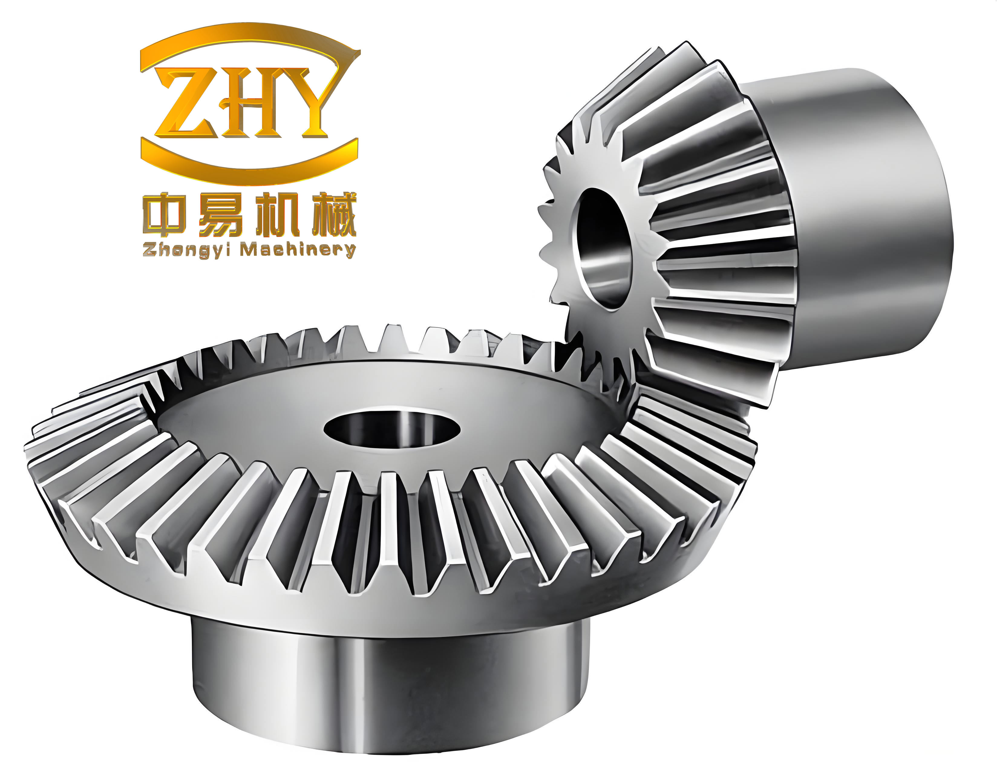
My modeling route is intended for precise straight bevel gear geometry. It avoids the common error of replacing the spherical involute with a planar involute on the back cone. It also remains general: by changing the module, tooth number, pressure angle, pitch cone angle, face width, and addendum parameters, I can produce a different straight bevel gear without rebuilding the mathematical derivation from the beginning.
Nomenclature and Basic Relations
| Symbol | Meaning | Unit or expression |
|---|---|---|
| \(m\) | Module of the straight bevel gear | mm |
| \(z\) | Number of teeth | dimensionless |
| \(\alpha\) | Pressure angle | degree or rad |
| \(\delta\) | Pitch cone angle | rad |
| \(\delta_b\) | Base cone angle | rad |
| \(\delta_a\) | Addendum cone angle | rad |
| \(\delta_f\) | Dedendum cone angle | rad |
| \(R\) | Pitch cone distance | mm |
| \(B\) | Face width | mm |
| \(\phi\) | Rolling parameter of the spherical involute | rad |
| \(\psi\) | Auxiliary angle in the moving coordinate system | rad |
| \(\theta_1\) | Angular offset from base cone to pitch cone | rad |
| \(\theta_2\) | Half-tooth angular offset at the pitch cone | rad |
| \(\theta\) | Total angular offset for the opposite tooth side | rad |
| \(Q_x,Q_y,Q_z\) | Right-side spherical involute coordinates in the fixed system | mm |
| \(P_x,P_y,P_z\) | Left-side spherical involute coordinates in the fixed system | mm |
For a straight bevel gear, I use the standard pitch cone relation
$$ \tan\delta = \frac{z_1}{z_2} $$
where \(z_1\) and \(z_2\) are the tooth numbers of the two mating straight bevel gears. For a single straight bevel gear, the pitch cone distance is
$$ R = \frac{m z}{2 \sin\delta} $$
The base cone angle follows from the pressure angle and the pitch cone angle:
$$ \sin\delta_b = \sin\delta \cos\alpha $$
The addendum and dedendum cone angles are
$$ \delta_a = \delta + \theta_a,\qquad \delta_f = \delta – \theta_f $$
where I define the addendum and dedendum angles by
$$ \theta_a = \arctan\frac{h_a}{R},\qquad \theta_f = \arctan\frac{h_f}{R} $$
For standard straight bevel gear proportions, \(h_a = m\) and \(h_f = 1.25m\) when a standard clearance is included. If a different addendum modification is used, I simply replace these values and continue with the same spherical involute formulation.
Generation Principle of the Spherical Involute
I begin from the theoretical generation principle of the straight bevel gear tooth surface. A generating plane is tangent to a base cone. The vertex of the base cone and the vertex of the pitch cone coincide at the same point. The generating plane rolls without sliding on the base cone. A straight line in the generating plane that passes through the cone vertex sweeps out the conical involute surface. When this surface is intersected by a sphere whose center is the cone vertex and whose radius is the cone distance, the intersection curve is the spherical involute. This spherical involute is the true profile of the straight bevel gear tooth on the big end.
I define a fixed coordinate system \(S(x,y,z)\). The origin is the cone vertex. The \(z\)-axis coincides with the axis of the straight bevel gear. The positive \(z\)-direction points from the vertex toward the large end. The \(x\)-axis lies along the radius that contains the starting point of the spherical involute. The \(y\)-axis is determined by the right-hand rule.
I also define a moving coordinate system \(S_1(x_1,y_1,z_1)\). It also has its origin at the cone vertex. The \(z_1\)-axis is the instantaneous rolling axis. The \(x_1\)-axis lies in the generating plane and is perpendicular to the \(z_1\)-axis. The \(y_1\)-axis is again determined by the right-hand rule.
At a given instant, a point \(K\) on the generating line has the following coordinates in the moving system:
$$ x_1 = R\sin\psi,\qquad y_1 = 0,\qquad z_1 = R\cos\psi $$
Because the generating plane rolls without sliding on the base cone, the arc length on the generating plane equals the arc length on the base cone. This pure rolling condition gives
$$ \psi R = \phi R \sin\delta_b $$
and therefore
$$ \psi = \phi \sin\delta_b $$
Substituting this result into the moving coordinates gives
$$ x_1 = R\sin(\phi\sin\delta_b),\qquad y_1 = 0,\qquad z_1 = R\cos(\phi\sin\delta_b) $$
The transformation from the moving system \(S_1\) to the fixed system \(S\) is performed by two matrices. I use
$$ M_1 =
\begin{bmatrix}
\sin\phi & \cos\phi & 0 & 0\\
-\cos\phi & \sin\phi & 0 & 0\\
0 & 0 & 1 & 0\\
0 & 0 & 0 & 1
\end{bmatrix}
$$
and
$$ M_2 =
\begin{bmatrix}
1 & 0 & 0 & 0\\
0 & \cos\delta_b & \sin\delta_b & 0\\
0 & -\sin\delta_b & \cos\delta_b & 0\\
0 & 0 & 0 & 1
\end{bmatrix}
$$
The coordinate transformation is therefore
$$
\begin{bmatrix}
x\\y\\z\\1
\end{bmatrix}
=
M_1 M_2
\begin{bmatrix}
x_1\\y_1\\z_1\\1
\end{bmatrix}
$$
After substituting the moving coordinates and carrying out the matrix multiplication, I obtain the right-side spherical involute of the big end of the straight bevel gear:
$$
\begin{aligned}
Q_x(\phi) &= R\left[\cos(\phi\sin\delta_b)\sin\delta_b\cos\phi + \sin(\phi\sin\delta_b)\sin\phi\right] \\
Q_y(\phi) &= R\left[\cos(\phi\sin\delta_b)\sin\delta_b\sin\phi – \sin(\phi\sin\delta_b)\cos\phi\right] \\
Q_z(\phi) &= R\cos(\phi\sin\delta_b)\cos\delta_b
\end{aligned}
$$
The parameter \(\phi\) is not arbitrary. It begins at the base cone and ends at the addendum cone. Therefore, I use the range
$$ 0 \le \phi \le \phi_{\max} $$
where
$$ \phi_{\max} = \frac{\arccos\left(\dfrac{\cos\delta_a}{\cos\delta_b}\right)}{\sin\delta_b} $$
This range ensures that the spherical involute extends exactly from the base cone to the addendum cone. It does not overshoot the tooth tip, and it does not stop before the full working profile is formed.
For the small end of the same straight bevel gear, the spherical involute lies on a smaller sphere. The sphere radius is \(R-B\), where \(B\) is the face width. Therefore, I replace \(R\) by \(R-B\) in the big-end equations. The small-end right-side spherical involute is
$$
\begin{aligned}
Q_{x,s}(\phi) &= (R-B)\left[\cos(\phi\sin\delta_b)\sin\delta_b\cos\phi + \sin(\phi\sin\delta_b)\sin\phi\right] \\
Q_{y,s}(\phi) &= (R-B)\left[\cos(\phi\sin\delta_b)\sin\delta_b\sin\phi – \sin(\phi\sin\delta_b)\cos\phi\right] \\
Q_{z,s}(\phi) &= (R-B)\cos(\phi\sin\delta_b)\cos\delta_b
\end{aligned}
$$
These equations describe one side of one tooth. To build the complete tooth, I must also generate the opposite side. The opposite side is not a simple mirror in the fixed system because the tooth is tapered and the spherical involute is generated on a cone. I therefore introduce an auxiliary coordinate system \(S_2(x_2,y_2,z_2)\). Its origin is again the cone vertex. Its \(z_2\)-axis coincides with the \(z\)-axis. Its \(x_2\)-axis is rotated from the \(x\)-axis by an angle \(\theta\). The \(y_2\)-axis lies in the horizontal plane.
The angle \(\theta\) has two contributions. The first contribution \(\theta_1\) is the angle from the base cone starting radius to the pitch cone radius. The second contribution \(\theta_2\) is the half-tooth angular thickness at the pitch cone. I compute \(\theta_1\) from the dot product of two radius vectors. The first vector is
$$ r_1 = (R\sin\delta_b,\;0,\;0) $$
The second vector is the projection of the pitch point onto the \(xy\)-plane. At the pitch cone, the parameter value is
$$ \phi_p = \frac{\arccos\left(\dfrac{\cos\delta}{\cos\delta_b}\right)}{\sin\delta_b} $$
The corresponding radius vector is
$$ r_2 = \left(Q_x(\phi_p),\;Q_y(\phi_p),\;0\right) $$
Therefore,
$$ \theta_1 = \arccos\left(\frac{Q_x(\phi_p)}{R\sin\delta}\right) $$
The second contribution is the half-tooth angular thickness at the pitch cone. The tooth thickness at the pitch cone of the big end is \(0.5\pi m\). The corresponding pitch radius on the sphere is \(R\sin\delta\). Hence,
$$ \theta_2 = \frac{\pi m}{4R\sin\delta} $$
The total angular offset is
$$ \theta = \theta_1 + \theta_2 $$
Using this offset, I express the right-side spherical involute in the auxiliary system \(S_2\) as
$$
\begin{aligned}
x_2 &= Q_x(\phi)\cos\theta + Q_y(\phi)\sin\theta \\
y_2 &= Q_y(\phi)\cos\theta – Q_x(\phi)\sin\theta \\
z_2 &= Q_z(\phi)
\end{aligned}
$$
The left side of the same tooth is symmetric to the right side about the \(x_2z_2\)-plane in the auxiliary system. Therefore, in \(S_2\), the left side has the same \(x_2\) and \(z_2\), but the sign of \(y_2\) is reversed. When I transform this mirrored profile back to the fixed system \(S\), I obtain the left-side spherical involute of the big end of the straight bevel gear:
$$
\begin{aligned}
P_x(\phi) &= Q_x(\phi)\cos(2\theta) + Q_y(\phi)\sin(2\theta) \\
P_y(\phi) &= Q_x(\phi)\sin(2\theta) – Q_y(\phi)\cos(2\theta) \\
P_z(\phi) &= Q_z(\phi)
\end{aligned}
$$
For the small end, I again replace \(R\) with \(R-B\) in \(Q_x\), \(Q_y\), and \(Q_z\). This gives the small-end left-side spherical involute. I now have four boundary curves for one tooth: big-end right side, big-end left side, small-end right side, and small-end left side. These four curves are the foundation of my precise straight bevel gear model.
Summary of the Mathematical Model
| Geometric feature | Equation | Parameter range |
|---|---|---|
| Pitch cone distance | \(R = \dfrac{m z}{2\sin\delta}\) | global |
| Base cone angle | \(\sin\delta_b = \sin\delta\cos\alpha\) | global |
| Addendum cone angle | \(\delta_a = \delta + \arctan(h_a/R)\) | global |
| Big-end right side | \(Q_x,Q_y,Q_z\) as derived above | \(0\le\phi\le\phi_{\max}\) |
| Big-end left side | \(P_x,P_y,P_z\) as derived above | \(0\le\phi\le\phi_{\max}\) |
| Small-end right side | Replace \(R\) by \(R-B\) in \(Q_x,Q_y,Q_z\) | \(0\le\phi\le\phi_{\max}\) |
| Small-end left side | Replace \(R\) by \(R-B\) in \(P_x,P_y,P_z\) | \(0\le\phi\le\phi_{\max}\) |
| Pitch parameter | \(\phi_p = \dfrac{\arccos(\cos\delta/\cos\delta_b)}{\sin\delta_b}\) | single value |
| Angular offset | \(\theta = \theta_1 + \theta_2\) | single value |
Numerical Discretization
I implement the mathematical model in a numerical environment. I divide the parameter interval \([0,\phi_{\max}]\) into \(N\) intervals. For each index \(i\), I set
$$ \phi_i = \frac{i}{N}\phi_{\max},\qquad i=0,1,2,\ldots,N $$
For each \(\phi_i\), I compute the four boundary points:
$$
\begin{aligned}
&\bigl(Q_x(\phi_i),Q_y(\phi_i),Q_z(\phi_i)\bigr), \\
&\bigl(P_x(\phi_i),P_y(\phi_i),P_z(\phi_i)\bigr), \\
&\bigl(Q_{x,s}(\phi_i),Q_{y,s}(\phi_i),Q_{z,s}(\phi_i)\bigr), \\
&\bigl(P_{x,s}(\phi_i),P_{y,s}(\phi_i),P_{z,s}(\phi_i)\bigr)
\end{aligned}
$$
I write these coordinates into a text file with three columns. Each row contains \(x\), \(y\), and \(z\). I use one file for each of the four spherical involutes. This file format is accepted directly by the curve-through-XYZ-points function in SolidWorks.
| Step | Operation | Result |
|---|---|---|
| 1 | Choose \(N\), for example \(N=200\) | Fine discretization of the spherical involute |
| 2 | Compute \(\phi_i = i\phi_{\max}/N\) | Parameter values along the profile |
| 3 | Evaluate \(Q_x,Q_y,Q_z\) | Big-end right-side points |
| 4 | Evaluate \(P_x,P_y,P_z\) | Big-end left-side points |
| 5 | Evaluate small-end equations with \(R-B\) | Small-end right-side and left-side points |
| 6 | Export four text files | Curve data for SolidWorks |
SolidWorks Curve Construction
Inside SolidWorks, I use the command sequence for a curve through XYZ points. I insert the text file for the big-end right-side spherical involute. I repeat this for the big-end left side, the small-end right side, and the small-end left side. At this stage, I have four 3D curves in the model space. These curves are not sketches on a plane. They lie on spherical surfaces and represent the true spherical involute of the straight bevel gear.
Next, I create the addendum arcs at the big end and the small end. The spherical involute ends at the addendum cone. The addendum cone intersects the sphere of radius \(R\) at the big end and the sphere of radius \(R-B\) at the small end. These intersections are circles. I draw the circular arc on each addendum cone section. The arc connects the right-side spherical involute to the left-side spherical involute. I then trim the spherical involutes with these arcs. This step produces a closed big-end tooth profile and a closed small-end tooth profile.
The addendum arc for the big end lies on the cone of angle \(\delta_a\) and on the sphere of radius \(R\). Its radius in the plane perpendicular to the axis is
$$ r_{a,\text{big}} = R\sin\delta_a $$
The addendum arc for the small end lies on the same cone but on the sphere of radius \(R-B\). Its radius is
$$ r_{a,\text{small}} = (R-B)\sin\delta_a $$
I use these radii to position the arcs correctly. The arc center is on the gear axis. The axial positions are
$$ z_{a,\text{big}} = R\cos\delta_a,\qquad z_{a,\text{small}} = (R-B)\cos\delta_a $$
These values ensure that the tooth tip is formed exactly at the addendum cone. They also make sure that the big-end and small-end tooth profiles remain on the correct spherical surfaces.
Boundary Surface Creation
After I have the closed big-end profile and the closed small-end profile, I create the tooth surface. I use the boundary surface command in SolidWorks. I select the big-end profile as one boundary and the small-end profile as the other boundary. I also select the corresponding side curves as guide curves. The boundary surface function then generates a smooth surface that connects the big-end spherical involute to the small-end spherical involute. I repeat this for the left side and the right side of the tooth. The result is a surface model of one complete tooth of the straight bevel gear.
| Surface element | First boundary | Second boundary | Guide curves |
|---|---|---|---|
| Right flank | Big-end right profile | Small-end right profile | Big-end and small-end right spherical involutes |
| Left flank | Big-end left profile | Small-end left profile | Big-end and small-end left spherical involutes |
| Tooth tip | Big-end addendum arc | Small-end addendum arc | Addendum cone surface |
| Tooth root | Big-end root arc | Small-end root arc | Root cone surface |
Because the tooth surface is a conical involute surface, the boundary surface method gives an accurate representation of the straight bevel gear tooth. I do not need to approximate the tooth flank with a ruled surface or with a planar involute. The boundary curves are the true spherical involutes, and the surface interpolates between them along the tooth width.
Conversion from Surface to Solid
The boundary surface creates a surface body. To convert it into a solid, I use the thicken command. I select the surface body and specify the material thickness. In many cases, I thicken the entire tooth surface inward toward the tooth center. This produces a solid tooth. I then check that the solid is watertight and that the tooth tip and tooth root are properly closed. If necessary, I add small fillets or chamfers at the tooth tip, but I keep the working flanks as the exact spherical involute surfaces.
| Operation | SolidWorks command | Purpose |
|---|---|---|
| Import points | Insert > Curve > Curve through XYZ points | Create spherical involute curves |
| Trim profile | 3D sketch trim or split | Obtain closed big-end and small-end tooth profiles |
| Create flank | Insert > Surface > Boundary Surface | Build one tooth surface |
| Convert to solid | Insert > Boss/Base > Thicken | Turn the surface into a solid tooth |
| Pattern tooth | Insert > Pattern/Mirror > Circular Pattern | Create all teeth of the straight bevel gear |
Circular Pattern and Final Straight Bevel Gear
I create the full straight bevel gear by a circular pattern. I select the gear axis as the pattern axis. I set the number of instances equal to the number of teeth \(z\). The angular spacing is
$$ \Delta \theta_{\text{tooth}} = \frac{2\pi}{z} $$
The pattern operation rotates the solid tooth around the gear axis and produces all teeth. Because the tooth geometry is exact and the pattern is uniform, the resulting straight bevel gear has correct tooth spacing, correct tooth thickness, and correct spherical involute flanks on every tooth.
I usually verify the final model by checking the following quantities:
| Check | Expected result | Method |
|---|---|---|
| Pitch cone angle | \(\delta\) as specified | Measure cone angle in the model |
| Base cone angle | \(\delta_b = \arcsin(\sin\delta\cos\alpha)\) | Compare with mathematical value |
| Tooth thickness at pitch cone | Approximately \(0.5\pi m\) | Measure arc length on the pitch sphere |
| Number of teeth | \(z\) | Count pattern instances |
| Face width | \(B\) | Measure axial length of tooth along cone |
| Spherical involute accuracy | Four curves match the derived equations | Compare point coordinates in SolidWorks |
Example Parameter Set
To illustrate the procedure, I choose a representative straight bevel gear. I use module \(m=4\,\text{mm}\), number of teeth \(z=25\), pressure angle \(\alpha=20^\circ\), pitch cone angle \(\delta=35^\circ\), and face width \(B=20\,\text{mm}\). I compute the derived quantities as follows.
| Quantity | Expression | Value |
|---|---|---|
| Module | \(m\) | 4 mm |
| Tooth number | \(z\) | 25 |
| Pressure angle | \(\alpha\) | 20° |
| Pitch cone angle | \(\delta\) | 35° |
| Face width | \(B\) | 20 mm |
| Pitch cone distance | \(R = m z/(2\sin\delta)\) | 87.17 mm |
| Base cone angle | \(\sin\delta_b = \sin\delta\cos\alpha\) | 32.60° |
| Addendum angle | \(\theta_a = \arctan(h_a/R)\) | 2.63° |
| Addendum cone angle | \(\delta_a = \delta + \theta_a\) | 37.63° |
| Maximum parameter | \(\phi_{\max} = \arccos(\cos\delta_a/\cos\delta_b)/\sin\delta_b\) | 0.644 rad |
| Pitch parameter | \(\phi_p = \arccos(\cos\delta/\cos\delta_b)/\sin\delta_b\) | 0.312 rad |
| Angular offset | \(\theta = \theta_1+\theta_2\) | 0.078 rad |
The numerical values in this table are not part of a lookup table in my method. They are computed from the same equations that drive the model. If I change any input, the table updates automatically. This is what makes the procedure useful for a parametric straight bevel gear.
Why the Boundary Surface Method Is More Accurate
The usual approximate method replaces the spherical involute with a planar involute on the back cone. The back cone is an imaginary cone that unrolls the pitch cone onto a plane. The planar involute on that plane is easy to draw, and it is widely used in simplified straight bevel gear models. However, the back-cone involute is not the true tooth profile. The error is small near the pitch point, but it grows toward the tooth tip and the tooth root. It also changes with the cone angle and the face width.
In my boundary surface method, the tooth flank is built directly from the spherical involute. The spherical involute is the exact intersection of the conical involute surface with the sphere. Therefore, the resulting straight bevel gear model has correct tooth action geometry. The difference is especially important for large cone angles, large modules, and wide face widths.
| Error source | Back-cone approximation | Boundary surface method |
|---|---|---|
| Tooth flank definition | Planar involute on back cone | Spherical involute on a sphere |
| Big-end profile | Approximate | Exact within the spherical involute formulation |
| Small-end profile | Often scaled or approximated | Exact by replacing \(R\) with \(R-B\) |
| Tooth tip | Approximate arc | Addendum cone arc on the correct sphere |
| Tooth width transition | May be linear or ruled | Boundary surface through true spherical involutes |
| Parametric generality | Limited | High |
| Suitability for precise analysis | Moderate | High |
Detailed Derivation of the Opposite Side
The opposite side of the tooth is the most delicate part of the straight bevel gear model. A simple mirror in the global coordinate system does not produce the correct spherical involute. I must mirror the profile in the auxiliary system \(S_2\), where the tooth is symmetric about the \(x_2z_2\)-plane. The reason is that the tooth thickness is defined at the pitch cone, and the angular offset \(\theta\) places the pitch point at the correct position. After mirroring in \(S_2\), I transform back to the fixed system \(S\). This yields the left-side expressions \(P_x\), \(P_y\), and \(P_z\).
The double-angle terms in the final expressions appear naturally from the rotation back to the fixed system. I can verify them by expanding the trigonometric identities:
$$ \cos(2\theta) = \cos^2\theta – \sin^2\theta $$
$$ \sin(2\theta) = 2\sin\theta\cos\theta $$
These identities confirm that the left-side expressions are consistent with a rotation by \(\theta\), a reflection, and a rotation back by \(\theta\). The result is a mathematically exact counterpart to the right-side spherical involute.
Parameter Range and Trimming
The parameter range \(\phi\in[0,\phi_{\max}]\) is essential. If I use a smaller range, the tooth is too short and does not reach the addendum cone. If I use a larger range, the spherical involute extends beyond the addendum cone and the tooth tip becomes incorrect. I therefore compute \(\phi_{\max}\) from the addendum cone angle. The equation
$$ \phi_{\max} = \frac{\arccos(\cos\delta_a/\cos\delta_b)}{\sin\delta_b} $$
is derived from the condition that the spherical involute reaches the addendum cone. At \(\phi=\phi_{\max}\), the \(z\)-coordinate of the spherical involute satisfies
$$ Q_z(\phi_{\max}) = R\cos\delta_a $$
This is exactly the axial coordinate of the addendum cone at the big end. For the small end, the same condition applies with \(R\) replaced by \(R-B\).
| Parameter value | Physical meaning | Coordinates |
|---|---|---|
| \(\phi=0\) | Base cone point | \(Q_x=R\sin\delta_b,\;Q_y=0,\;Q_z=R\cos\delta_b\) |
| \(\phi=\phi_p\) | Pitch cone point | \(Q_x,Q_y\) at pitch radius; \(Q_z=R\cos\delta\) |
| \(\phi=\phi_{\max}\) | Addendum cone point | \(Q_x,Q_y\) at tip circle; \(Q_z=R\cos\delta_a\) |
Implementation Details in SolidWorks
I pay attention to the following implementation details when I build the straight bevel gear in SolidWorks:
First, I make sure that the coordinate system in the text file matches the SolidWorks coordinate system. I usually place the cone vertex at the origin and align the gear axis with the \(z\)-axis. If the SolidWorks model uses a different orientation, I apply a coordinate transformation before importing the points.
Second, I use a sufficiently large number of points. A typical value is \(N=200\) to \(N=400\). Too few points produce visible facets along the spherical involute. Too many points increase file size and may slow down the boundary surface operation without a visible improvement.
Third, I create the big-end and small-end profiles as closed curves before making the boundary surface. The boundary surface command works best when the two boundary curves have the same number of segments and are ordered consistently. I therefore generate the same number of points for the big end and the small end.
Fourth, I check the direction of the curves. If the boundary curves are reversed, the boundary surface may twist. I use the curve direction display in SolidWorks and reverse the curve if necessary.
Fifth, I use the thicken command with a small thickness or with a surface offset that matches the intended tooth solid. If the tooth is to be used in a finite element analysis, I may keep the flanks as surfaces and mesh them directly. If the tooth is to be used in a mechanical assembly, I thicken it into a solid and pattern it.
| Implementation issue | Symptom | Solution |
|---|---|---|
| Incorrect coordinate alignment | Tooth appears rotated or displaced | Match the cone vertex and gear axis in the text file |
| Too few points | Faceted spherical involute | Increase \(N\) |
| Unequal point counts | Boundary surface distortion | Use the same number of points on both ends |
| Reversed curve direction | Twisted tooth flank | Reverse the curve direction |
| Incorrect trimming arc | Tooth tip is open or too long | Use the addendum cone radius and axial position |
Parametric Behavior of the Straight Bevel Gear Model
I can study how the straight bevel gear model changes when I vary the input parameters. The following table summarizes the main trends.
| Input parameter | Effect on \(R\) | Effect on \(\delta_b\) | Effect on tooth shape |
|---|---|---|---|
| Module \(m\) increases | Increases linearly | No change | Larger tooth size |
| Tooth number \(z\) increases | Increases linearly for fixed \(\delta\) | No change | More teeth, smaller angular pitch |
| Pressure angle \(\alpha\) increases | No change | Decreases | Wider base cone, different involute curvature |
| Pitch cone angle \(\delta\) increases | Decreases for fixed \(m,z\) | Increases | Tooth becomes more steeply conical |
| Face width \(B\) increases | No change | No change | Small end becomes smaller; tooth taper is stronger |
| Addendum \(h_a\) increases | No change | No change | Tooth tip extends further outward |
This parametric behavior is important because it shows that the boundary surface method is not restricted to one particular straight bevel gear. I can use the same mathematical model for different modules, tooth numbers, pressure angles, and cone angles. I only need to update the input parameters and recompute the point coordinates.
Comparison with Other Modeling Strategies
I have also compared my method with other common strategies for straight bevel gear modeling. A swept cut or a lofted cut can create a tooth-like shape, but it does not guarantee a spherical involute. A simple extrusion followed by a taper is even less accurate. A back-cone approximation is better, but it still introduces geometric error. My boundary surface method is more accurate because it uses the spherical involute as the boundary of the surface.
| Method | Tooth flank accuracy | Parametric flexibility | Implementation effort |
|---|---|---|---|
| Extrude with taper | Low | Low | Low |
| Swept cut | Low to moderate | Moderate | Moderate |
| Lofted cut | Moderate | Moderate | Moderate |
| Back-cone involute | Moderate | Moderate | Moderate |
| Boundary surface with spherical involute | High | High | Moderate to high |
Mathematical Summary of the Complete Tooth
I summarize the complete tooth formulation in one table. This table is the core reference that I use when I generate the straight bevel gear model.
| Curve | Coordinates | Notes |
|---|---|---|
| Big-end right | \(Q_x(\phi),\;Q_y(\phi),\;Q_z(\phi)\) | Use \(R\) |
| Big-end left | \(P_x(\phi),\;P_y(\phi),\;P_z(\phi)\) | Use \(R\) and \(\theta\) |
| Small-end right | \(Q_{x,s}(\phi),\;Q_{y,s}(\phi),\;Q_{z,s}(\phi)\) | Replace \(R\) by \(R-B\) |
| Small-end left | \(P_{x,s}(\phi),\;P_{y,s}(\phi),\;P_{z,s}(\phi)\) | Replace \(R\) by \(R-B\) in \(P_x,P_y,P_z\) |
| Big-end addendum arc | Circle on sphere \(R\), cone \(\delta_a\) | Radius \(R\sin\delta_a\) |
| Small-end addendum arc | Circle on sphere \(R-B\), cone \(\delta_a\) | Radius \((R-B)\sin\delta_a\) |
Numerical Accuracy and Convergence
Because the method is numerical, I also consider convergence. As I increase the number of points \(N\), the polyline approximation of the spherical involute converges to the exact curve. The boundary surface becomes smoother. The tooth solid becomes more accurate. I can estimate the chord error for a given \(N\). If the arc length of the spherical involute is \(L\), the approximate chord error for a uniform discretization is of order
$$ e_{\text{chord}} \sim \frac{L^2}{8N^2 \rho} $$
where \(\rho\) is a representative radius of curvature. In practice, I find that \(N=200\) is sufficient for most straight bevel gear models. For high-precision applications, I use \(N=400\) or more.
| Number of points \(N\) | Relative chord error | Recommended use |
|---|---|---|
| 50 | High | Conceptual visualization only |
| 100 | Moderate | Preliminary design |
| 200 | Low | General precise modeling |
| 400 | Very low | High-precision analysis |
| 800 | Negligible | Reference geometry |
Applying the Model to a Complete Straight Bevel Gear Pair
I can extend the same method to a pair of straight bevel gears. For a pair with shaft angle \(90^\circ\), the pitch cone angles satisfy
$$ \delta_1 + \delta_2 = 90^\circ $$
and
$$ \tan\delta_1 = \frac{z_1}{z_2},\qquad \tan\delta_2 = \frac{z_2}{z_1} $$
I build each straight bevel gear separately using the same spherical involute method. I then assemble them with the correct cone distance and the correct axial positioning. The resulting assembly has exact spherical involute flanks, and I can use it for motion simulation, contact analysis, or manufacturing preparation.
For a straight bevel gear pair, I also check the following conditions:
| Condition | Expression | Purpose |
|---|---|---|
| Shaft angle | \(\Sigma = \delta_1 + \delta_2\) | Confirm assembly angle |
| Gear ratio | \(i = z_2/z_1\) | Confirm kinematic ratio |
| Pitch cone distance equality | \(R_1 = R_2\) | Confirm mesh alignment |
| Tooth thickness compatibility | \(s_1 + s_2 = \pi m\) | Confirm backlash-free theoretical mesh |
Manufacturing and Analysis Implications
The precise straight bevel gear model is useful beyond visualization. I can export the model to a CAM environment and use it to generate toolpaths for a five-axis machine. I can also import it into a finite element analysis package to study contact stress and bending stress. Because the tooth flanks are true spherical involutes, the analysis results are more reliable than those obtained from an approximate model.
In my experience, the boundary surface method is especially valuable when the straight bevel gear has a large cone angle, a large module, or a wide face width. In these cases, the difference between the spherical involute and the back-cone approximation becomes significant. The precise model reduces the risk of interference and improves the prediction of the contact pattern.
| Application | Benefit of precise straight bevel gear model |
|---|---|
| CAD assembly | Correct geometry and no visual interference |
| Motion simulation | Accurate kinematic behavior |
| Finite element analysis | Realistic contact and stress distribution |
| CAM programming | Accurate toolpath generation |
| Inspection planning | Correct nominal coordinates for measurement |
| Reverse engineering | Comparison standard for scanned straight bevel gears |
Step-by-Step Procedure I Follow
For clarity, I list the complete procedure that I use to model a straight bevel gear with the boundary surface method.
| Step | Action | Details |
|---|---|---|
| 1 | Define input parameters | \(m,z,\alpha,\delta,B,h_a,h_f\) |
| 2 | Compute derived angles and distances | \(R,\delta_b,\delta_a,\delta_f,\phi_{\max},\phi_p,\theta_1,\theta_2,\theta\) |
| 3 | Discretize \(\phi\) | \(\phi_i = i\phi_{\max}/N\) |
| 4 | Evaluate big-end right and left spherical involutes | Use \(Q_x,Q_y,Q_z\) and \(P_x,P_y,P_z\) |
| 5 | Evaluate small-end right and left spherical involutes | Replace \(R\) by \(R-B\) |
| 6 | Export XYZ point files | One file for each curve |
| 7 | Insert curves into SolidWorks | Curve through XYZ points |
| 8 | Create addendum arcs | Big-end and small-end cone sections |
| 9 | Trim spherical involutes | Close the tooth profiles |
| 10 | Create boundary surfaces | Right flank, left flank, tip, root |
| 11 | Thicken surface to solid | Create one tooth |
| 12 | Circular pattern | \(z\) instances around the gear axis |
| 13 | Validate model | Check angles, tooth thickness, and pattern |
Mathematical Checks and Validation Formulas
I use several formulas to validate the straight bevel gear model after it is built. These checks help me confirm that the spherical involute has been implemented correctly.
The pitch point on the big-end spherical involute should satisfy
$$ Q_z(\phi_p) = R\cos\delta $$
The addendum point on the big-end spherical involute should satisfy
$$ Q_z(\phi_{\max}) = R\cos\delta_a $$
The base point on the big-end spherical involute should satisfy
$$ Q_x(0) = R\sin\delta_b,\qquad Q_y(0)=0,\qquad Q_z(0)=R\cos\delta_b $$
The small-end counterparts follow by replacing \(R\) with \(R-B\). These checks are simple, but they catch most coordinate transformation errors.
| Check point | Big-end condition | Small-end condition |
|---|---|---|
| Base point | \(z=R\cos\delta_b\) | \(z=(R-B)\cos\delta_b\) |
| Pitch point | \(z=R\cos\delta\) | \(z=(R-B)\cos\delta\) |
| Addendum point | \(z=R\cos\delta_a\) | \(z=(R-B)\cos\delta_a\) |
| Radial distance at pitch | \(\sqrt{Q_x^2+Q_y^2}=R\sin\delta\) | \(\sqrt{Q_x^2+Q_y^2}=(R-B)\sin\delta\) |
| Radial distance at addendum | \(\sqrt{Q_x^2+Q_y^2}=R\sin\delta_a\) | \(\sqrt{Q_x^2+Q_y^2}=(R-B)\sin\delta_a\) |
Advantages of the Boundary Surface Method for Straight Bevel Gears
The method I describe has several advantages. First, it is mathematically exact with respect to the spherical involute. Second, it is fully parametric: I can change the input parameters and regenerate the point files. Third, it uses standard SolidWorks commands, so I do not need a specialized gear design package. Fourth, it produces a solid model that is suitable for assembly and analysis. Fifth, it avoids the geometric errors of the back-cone approximation. Sixth, it handles both the big end and the small end correctly. Seventh, it can be extended to other types of bevel gears with appropriate modifications.
| Advantage | Explanation |
|---|---|
| Exact spherical involute | Flanks are generated from the true tooth surface |
| Parametric regeneration | Input changes update the entire model |
| Standard CAD tools | No specialized add-in is required |
| Solid output | Ready for assembly, simulation, and manufacturing |
| Big-end and small-end consistency | Both ends use the same mathematical model |
| Good for large cone angles | Errors of back-cone approximation are avoided |
Limitations and Practical Considerations
I also recognize the limitations of the method. The first limitation is that it requires numerical computation. I need a script or a spreadsheet to evaluate the spherical involute equations. The second limitation is that the boundary surface may require careful curve matching. If the curves are not ordered consistently, the surface can twist. The third limitation is that the thicken operation may fail if the surface has very small features or sharp corners. I usually repair these areas with small fillets or by adjusting the root geometry. The fourth limitation is that the method does not automatically include manufacturing features such as root fillets, chamfers, or crowning. I add those features after the basic straight bevel gear tooth is built.
| Limitation | Practical solution |
|---|---|
| Requires numerical evaluation | Use a script or a parametric spreadsheet |
| Curve direction sensitivity | Check and reverse curve directions in SolidWorks |
| Thicken failures | Simplify small details or adjust surface offset |
| No automatic root fillet | Add fillet after solid creation |
| No crowning | Apply local surface modification if needed |
Final Remarks
I have presented a precise three-dimensional modeling method for straight bevel gears. The method starts from the generation principle of the conical involute surface and derives the spherical involute equations for both sides of the tooth and for both the big end and the small end. I discretize the spherical involute, export the coordinates to SolidWorks, create the curves through XYZ points, trim them with the addendum cone arcs, build the tooth surfaces with the boundary surface command, convert the surfaces to a solid, and complete the straight bevel gear with a circular pattern. The result is a straight bevel gear model that is more accurate than the common back-cone approximation and more flexible than a purely manual CAD construction. I can reuse the same equations for different straight bevel gear parameters, and I can apply the model to assembly, kinematic simulation, finite element analysis, and manufacturing preparation.
In my workflow, the most important idea is that the straight bevel gear tooth is not a planar involute. It is a spherical involute. Once I treat it as a spherical involute, the big-end and small-end profiles, the opposite tooth side, and the tooth tip all become consistent. The boundary surface method then turns that mathematical consistency into a solid model inside SolidWorks. For any straight bevel gear, the same sequence applies: derive, discretize, export, insert, trim, surface, thicken, and pattern. This sequence is the core of my precise straight bevel gear modeling approach.