
I study the coupled transition behavior of straight bevel gears when backlash, time-varying mesh stiffness, and rotational speed interact. My focus is not only on the existence of periodic motion, but also on how periodic motion changes into tooth-surface impact, non-meshing, tooth-back contact, and dynamic load amplification. In straight bevel gears, these phenomena are strongly coupled because the mesh force depends on the instantaneous dynamic transmission error, the backlash function, and the time-varying mesh stiffness. I therefore construct a two-parameter solution-domain structure in the plane of the time-varying mesh stiffness coefficient and the frequency ratio. The resulting structures allow me to see where straight bevel gears operate in a safe meshing state, where unilateral impact appears, where bilateral impact appears, and where chaotic or quasi-periodic motion dominates. The main tools I use are cell mapping, the continuous-Poincaré-Newton-Floquet method, Floquet multiplier tracking, and continuation of periodic solutions. I also quantify non-meshing duty, back-meshing duty, and dynamic load coefficient so that the parameter-domain boundaries are not merely topological but also physically meaningful for straight bevel gears.
1. Physical Model of Straight Bevel Gears
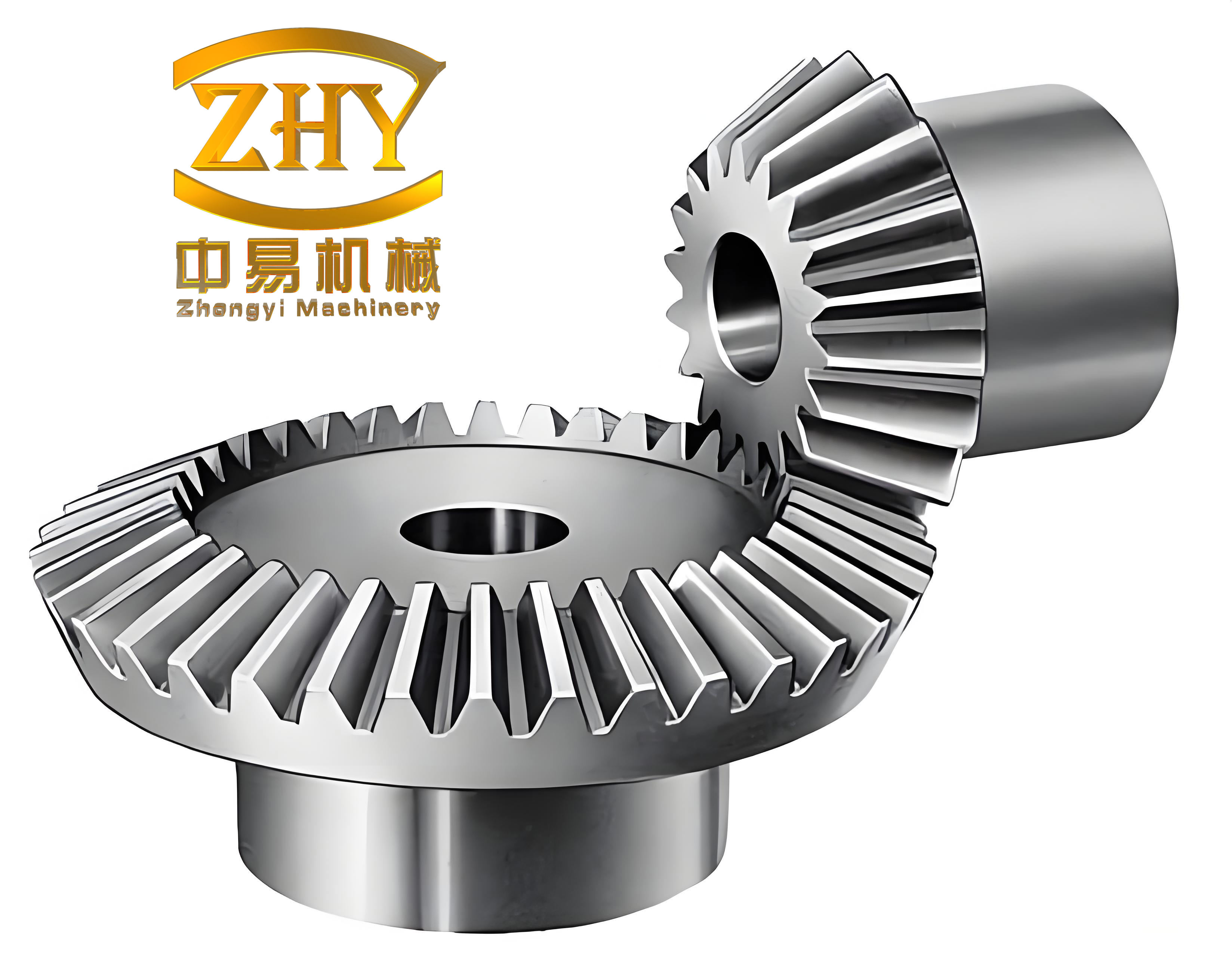
I consider a straight bevel gear pair supported elastically, with two orthogonal axes intersecting at the origin. The two gear bodies are treated as rigid conical disks. Their elastic supports are represented at the mid-face positions along the coordinate axes. The support stiffness and damping are denoted by \(k_{ij}\) and \(c_{ij}\), where the first index identifies the coordinate direction and the second index identifies the gear. The mesh damping is \(c_h\), the time-varying mesh stiffness is \(k_h(t)\), and the backlash is \(b_h\). The driving torque applied to the driving gear consists of a constant part and a fluctuating part, while the driven gear is subjected to a constant resistant torque. I neglect swinging and bending of the shafts, so the vibration of the two rigid conical disks consists of translations along the coordinate axes and rotations about their own axes. After I merge the two rotational coordinates into the dynamic transmission error, the governing system becomes a strongly nonlinear, piecewise-smooth, parametrically excited model of straight bevel gears.
I define the dynamic transmission error along the mesh line as
$$
\Lambda_n = (X_1-X_2)a_1 – (Y_1-Y_2)a_2 – (Z_1+r_1\theta_1-Z_2-r_2\theta_2)a_3 – e_n(t),
$$
where \(X_j\), \(Y_j\), and \(Z_j\) are translational displacements, \(\theta_j\) are angular displacements, \(r_j\) are pitch radii, \(e_n(t)\) is the static transmission error, and the geometric coefficients are
$$
a_1=\cos\delta_1\sin\alpha_n,\qquad
a_2=\cos\delta_1\cos\alpha_n,\qquad
a_3=\cos\alpha_n.
$$
Here, \(\delta_1\) is the pitch cone angle of the driving straight bevel gear and \(\alpha_n\) is the normal pressure angle. The static transmission error is expanded as a Fourier series:
$$
e_n(t)=\sum_{l=1}^{N} A_l\cos(l\Omega_h t+\Phi_l),
$$
where \(\Omega_h\) is the mesh frequency, \(A_l\) is the harmonic amplitude, and \(\Phi_l\) is the initial phase. For straight bevel gears in practical transmission systems, the first harmonic often dominates the mesh excitation, but I retain the series form because higher harmonics can influence impact timing when backlash is present.
The normal mesh force is written as
$$
F_n = k_h(t) f(\Lambda_n)+c_h\dot{\Lambda}_n.
$$
Its components along the coordinate axes are
$$
F_x=-a_4F_n,\qquad
F_y=a_5F_n,\qquad
F_z=a_3F_n,
$$
with
$$
a_4=\sin\alpha_n\cos\delta_1+\cos\alpha_n\sin\delta_1,
\qquad
a_5=\sin\alpha_n\sin\delta_1-\cos\alpha_n\cos\delta_1.
$$
The time-varying mesh stiffness of straight bevel gears is expanded as
$$
k_h(t)=k_m+\sum_{l=1}^{N} k_{kl}\cos(l\Omega_h t+\Phi_{kl}),
$$
where \(k_m\) is the mean mesh stiffness, \(k_{kl}\) is the harmonic amplitude, and \(\Phi_{kl}\) is the phase. In my nondimensional formulation, I use
$$
k_h(\tau)=1+\alpha\cos(\Omega\tau),
$$
where \(\alpha\) is the time-varying mesh stiffness coefficient and \(\Omega\) is the frequency ratio. The coefficient \(\alpha\) measures the unevenness of single-tooth and double-tooth meshing in straight bevel gears. The frequency ratio \(\Omega\) measures the relationship between the mesh frequency and the natural frequency.
The backlash function is piecewise smooth and is given by
$$
f(\Lambda_n)=
\begin{cases}
\Lambda_n-b_h, & \Lambda_n>b_h,\\
0, & |\Lambda_n|\le b_h,\\
\Lambda_n+b_h, & \Lambda_n<-b_h.
\end{cases}
$$
This piecewise function is the source of the non-smooth dynamics in straight bevel gears. When the dynamic transmission error falls inside the backlash interval, the teeth lose contact. When it exceeds the positive backlash limit, the tooth surfaces mesh. When it falls below the negative backlash limit, the tooth backs contact. Therefore, the same straight bevel gear pair can exhibit driving-side meshing, non-meshing, unilateral impact, and bilateral impact within one periodic cycle.
2. Nondimensional Equations of Motion
I nondimensionalize the displacements by a nominal backlash \(b_n\), and I introduce the natural frequency
$$
\Omega_n=\left(\frac{k_m}{m_e}\right)^{1/2},
$$
where the equivalent mass of the straight bevel gear pair is
$$
m_e=\frac{J_1J_2}{r_1^2J_2+r_2^2J_1}.
$$
I also define the nondimensional time \(\tau=\Omega t\), the frequency ratio \(\Omega=\Omega_h/\Omega_n\), and the nondimensional dynamic transmission error \(\lambda=\Lambda_n/b_n\). The nondimensional support and mesh parameters are
$$
\xi_{ij}=\frac{c_{ij}}{2m_j\Omega_n},\qquad
k_{ij}=\left(\frac{\Omega_{ij}}{\Omega_n}\right)^2,\qquad
\xi_{hj}=\frac{c_h}{2m_j\Omega_n},\qquad
\xi_h=\frac{c_h}{2m_e\Omega_n}.
$$
After algebraic manipulation, the nondimensional equations of motion for the straight bevel gear system become
$$
\begin{aligned}
\ddot{x}_1+2\xi_{x1}\dot{x}_1+2a_4\xi_{h1}\dot{\lambda}+k_{x1}x_1+a_4 k_{h1}f(\lambda)&=0,\\
\ddot{y}_1+2\xi_{y1}\dot{y}_1-2a_5\xi_{h1}\dot{\lambda}+k_{y1}y_1-a_5 k_{h1}f(\lambda)&=0,\\
\ddot{z}_1+2\xi_{z1}\dot{z}_1-2a_3\xi_{h1}\dot{\lambda}+k_{z1}z_1-a_3 k_{h1}f(\lambda)&=0,\\
\ddot{x}_2+2\xi_{x2}\dot{x}_2-2a_4\xi_{h2}\dot{\lambda}+k_{x2}x_2-a_4 k_{h2}f(\lambda)&=0,\\
\ddot{y}_2+2\xi_{y2}\dot{y}_2+2a_5\xi_{h2}\dot{\lambda}+k_{y2}y_2+a_5 k_{h2}f(\lambda)&=0,\\
\ddot{z}_2+2\xi_{z2}\dot{z}_2+2a_3\xi_{h2}\dot{\lambda}+k_{z2}z_2+a_3 k_{h2}f(\lambda)&=0,\\
-a_1x_1+a_2y_1+a_3z_1+a_1x_2-a_2y_2-a_3z_2+\ddot{\lambda}+2a_3\xi_h\dot{\lambda}+a_3k_h f(\lambda)&=f_{pm}+f_{pv}+f_e\Omega^2\cos(\Omega\tau).
\end{aligned}
$$
I collect the state variables as
$$
\mathbf{X}=
\begin{bmatrix}
x_1 & \dot{x}_1 & y_1 & \dot{y}_1 & z_1 & \dot{z}_1 &
x_2 & \dot{x}_2 & y_2 & \dot{y}_2 & z_2 & \dot{z}_2 & \lambda & \dot{\lambda}
\end{bmatrix}^{T}.
$$
The system can then be written in compact first-order form as
$$
\frac{d\mathbf{X}}{d\tau}=\mathbf{F}(\mathbf{X},\tau;\Omega,\alpha),
\qquad
\mathbf{F}(\mathbf{X},\tau;\Omega,\alpha)=\mathbf{F}(\mathbf{X},\tau+T;\Omega,\alpha),
$$
where \(T\) is the nondimensional period of the parametric excitation. This periodic forcing is essential because the stability of straight bevel gears is not determined by a single equilibrium but by the stability of periodic orbits in the parameter plane.
| Symbol | Meaning in straight bevel gears | Typical nondimensional value |
|---|---|---|
| \(\xi_{i1},\xi_{i2}\) | Support damping ratios in \(x,y,z\) directions | \(0.01\) |
| \(\xi_{h1},\xi_{h2}\) | Mesh damping ratios with respect to each gear | \(0.0125\) |
| \(\xi_h\) | Equivalent mesh damping ratio | \(0.05\) |
| \(k_{i1},k_{i2}\) | Support stiffness parameters | \(1.0\) |
| \(k_{h1},k_{h2}\) | Mesh stiffness scaling parameters | \(0.5\) |
| \(f_{pm}\) | Nondimensional mean driving force | \(0.5\) |
| \(f_e\) | Nondimensional transmission error amplitude | \(0.2\) |
| \(b\) | Nondimensional backlash | \(1.0\) |
| \(\alpha\) | Time-varying mesh stiffness coefficient | \(0.05\) to \(0.55\) |
| \(\Omega\) | Frequency ratio | \(1.2\) to \(1.7\) |
3. Impact, Non-Meshing, and Dynamic Load Metrics
For straight bevel gears with backlash, the impact state within one periodic cycle can be classified using the minimum dynamic transmission error \(\lambda_{\min}\). I define the impact index \(I\) as
$$
I=
\begin{cases}
0, & \lambda_{\min}>b \quad \text{no impact, meshing},\\
0, & \lambda_{\min}=b \quad \text{tooth-surface friction slide, meshing},\\
1, & -b<\lambda_{\min}<b $$="" &="" 1,="" 2,="" <p="" \end{cases}="" \lambda_{\min}="-b" \lambda_{\min}This classification is important for straight bevel gears because the machine may still rotate while the teeth are not transmitting load on the intended driving side. I use three scalar metrics to quantify the severity of these states. The non-meshing duty coefficient is
$$
\delta_{\mathrm{NMDC}}=\frac{t_1}{T},
$$
where \(t_1\) is the time spent in a non-meshing condition during one cycle. The back-meshing duty coefficient is
$$
\delta_{\mathrm{BMDC}}=\frac{t_2}{T},
$$
where \(t_2\) is the time spent in tooth-back meshing. The dynamic load coefficient is
$$
\delta_{\mathrm{DLC}}=\frac{\max |f_n(\tau)|}{f_{pm}},
$$
where \(f_n(\tau)\) is the nondimensional normal mesh force and \(f_{pm}\) is the mean driving force. For straight bevel gears, these three metrics give a direct picture of how bifurcation and impact transitions couple to practical vibration and load problems.
| Metric | Physical interpretation | Desired direction |
|---|---|---|
| \(\delta_{\mathrm{NMDC}}\) | Fraction of cycle without proper driving-side meshing | As small as possible |
| \(\delta_{\mathrm{BMDC}}\) | Fraction of cycle with tooth-back contact | As small as possible |
| \(\delta_{\mathrm{DLC}}\) | Peak normal force divided by mean force | Close to unity |
| \(I=0\) | No impact or only sliding contact on the driving surface | Preferred |
| \(I=1\) | Unilateral impact and partial non-meshing | Acceptable only in limited ranges |
| \(I=2\) | Bilateral impact and tooth-back meshing | Avoid |
4. Parametric Solution-Domain Method for Straight Bevel Gears
I use a cell-mapping framework to construct the parameter-domain structure of straight bevel gears. I select the frequency ratio \(\Omega\) and the time-varying mesh stiffness coefficient \(\alpha\) as the two control parameters. The parameter plane is
$$
\Theta=[\Omega_l,\Omega_u]\times[\alpha_l,\alpha_u]=[1.2,1.7]\times[0.05,0.55].
$$
I discretize this plane into \(501\times501\) cells. Each cell represents a small parameter combination. For each cell, I solve for the periodic response and then continue the periodic orbit along the parameter directions. This cell-based continuation allows me to capture the solution-domain boundaries of straight bevel gears without losing the global topology of periodic, quasi-periodic, and chaotic regions.
Let the cell sizes in the \(\Omega\) and \(\alpha\) directions be
$$
h_{\Omega}=\frac{\Omega_u-\Omega_l}{n},
\qquad
h_{\alpha}=\frac{\alpha_u-\alpha_l}{m}.
$$
The parameter values in the cells are
$$
\Omega_i=\Omega_l+i h_{\Omega},\qquad
\alpha_j=\alpha_l+j h_{\alpha},
$$
where \(i=1,2,\dots,n\) and \(j=1,2,\dots,m\). I then store the response type, impact index, non-meshing duty, back-meshing duty, and dynamic load coefficient for each cell.
| Step | Operation in my solution-domain algorithm | Output |
|---|---|---|
| 1 | Discretize the \(\Omega\times\alpha\) plane into cells | Parameter grid |
| 2 | Solve for a periodic orbit in the first cell using a pseudo-fixed-point method | Initial periodic solution |
| 3 | Track the orbit with the continuous-Poincaré-Newton-Floquet method | Continued periodic branch |
| 4 | Compute Floquet multipliers and test \(|\lambda|_{\max}\) | Stability and bifurcation points |
| 5 | If the orbit loses stability, classify the bifurcation and restart the periodic search | New periodic branch or chaotic state |
| 6 | Record impact index \(I\) and period \(P\) in every cell | \(I/P\) solution-domain structure |
| 7 | Compute \(\delta_{\mathrm{NMDC}}\), \(\delta_{\mathrm{BMDC}}\), and \(\delta_{\mathrm{DLC}}\) | Physical property maps |
The continuous-Poincaré-Newton-Floquet method solves the periodicity condition directly. I integrate the state equation and the variational equation over one period:
$$
\frac{d\mathbf{X}}{d\tau}=\mathbf{F}(\mathbf{X},\tau),
\qquad
\frac{d\Phi}{d\tau}=\frac{\partial\mathbf{F}}{\partial\mathbf{X}}\Phi,
$$
where \(\Phi\) is the transition matrix. The Floquet multipliers are the eigenvalues of \(\Phi(T)\). A periodic orbit of straight bevel gears is stable if
$$
\max_i |\lambda_i|<1.
$$
When a multiplier crosses the unit circle, the stability changes. A real multiplier crossing \(+1\) usually corresponds to a saddle-node or grazing-related transition. A real multiplier crossing \(-1\) corresponds to period doubling. A pair of complex multipliers crossing the unit circle corresponds to a Hopf bifurcation, which in my straight bevel gear model leads to quasi-periodic or torus-like motion.
For continuation, I use the prediction
$$
\mathbf{X}_{k+1,0}
=
\mathbf{X}_k
–
\left[G_{\mathbf{X}}(\Omega_k,\mathbf{X}_k)\right]^{-1}
G_{\Omega}(\Omega_k,\mathbf{X}_k)\Delta\Omega,
\qquad
\Omega_{k+1}=\Omega_k+\Delta\Omega,
$$
where
$$
G_{\mathbf{X}}=\mathbf{I}-D P(\Omega_k,\mathbf{X}_k),
\qquad
G_{\Omega}=P_{\Omega}(\Omega_k,\mathbf{X}_k).
$$
The term \(P_{\Omega}\) is obtained by integrating the sensitivity equation
$$
\frac{dP_{\Omega}}{d\tau}
=
\frac{\partial\mathbf{F}}{\partial\mathbf{X}}P_{\Omega}
+
\frac{\partial\mathbf{F}}{\partial\Omega}.
$$
This sensitivity-based continuation is efficient for straight bevel gears because it avoids computing long chaotic transients when only the periodic branch is needed.
5. Bifurcation Modes in Straight Bevel Gears
In my solution-domain structures, I observe several bifurcation modes in straight bevel gears. These modes are not isolated mathematical events; they organize the boundaries between periodic, quasi-periodic, and chaotic regions. I summarize the main modes in the following table.
| Bifurcation mode | Floquet condition | Typical response transition in straight bevel gears |
|---|---|---|
| Saddle-node bifurcation | Real multiplier crosses \(+1\) | Birth or disappearance of a periodic branch |
| Period-doubling bifurcation | Real multiplier crosses \(-1\) | \(P\rightarrow 2P\rightarrow 4P\rightarrow\cdots\) |
| Hopf bifurcation | Complex multiplier pair crosses the unit circle | Periodic to quasi-periodic motion |
| Period-3 bifurcation | Periodic solution with \(P=3\) is created | \(P=1\rightarrow P=3\), \(P=3\rightarrow 3P\) |
| Catastrophe | Sudden change of attractor size or basin | Periodic to chaotic or chaotic to periodic |
| Grazing bifurcation | Orbit touches \(\lambda=\pm b\) | Impact state changes without simple multiplier crossing |
The impact state of straight bevel gears changes when the periodic orbit touches the backlash boundaries \(\lambda=b\) or \(\lambda=-b\). This is a non-smooth bifurcation. It can create or destroy unilateral impact and bilateral impact even when the smooth Floquet multiplier criterion does not show a simple crossing. For this reason, I combine Floquet analysis with the impact index \(I\). If a real multiplier crosses the unit circle at the same time as the orbit touches a backlash boundary, I classify the event as a saddle-node-like transition. If the orbit touches the boundary without such a multiplier crossing, I classify it as a grazing event.
6. Solution-Domain Structure in the Frequency-Ratio and Stiffness Plane
I construct the \(I/P\) solution-domain structure for straight bevel gears in the \(\Omega\times\alpha\) plane. The notation \(I/P\) means impact index over period. For example, \(0/1\) denotes no impact with period 1, \(1/1\) denotes unilateral impact with period 1, \(2/1\) denotes bilateral impact with period 1, and \(1/N\) denotes unilateral impact with long-period, quasi-periodic, or chaotic motion. I summarize the main regions below.
| Region | Parameter range | Dominant bifurcations | Typical \(I/P\) states |
|---|---|---|---|
| Low stiffness region | \(\alpha<0.15\) | Saddle-node, period-3 | \(0/1\), \(1/1\), \(1/3\) |
| Intermediate stiffness region | \(0.15<\alpha<0.30\) | Period-doubling, period-3, Hopf | \(1/1\), \(1/3\), quasi-periodic, chaos |
| High stiffness region | \(0.30<\alpha<0.55\) | Grazing, period-3, catastrophe | \(2/1\), \(2/3\), \(2/N\), chaos |
| Low frequency-ratio region | \(\Omega<1.25\) | Impact transitions in \(P=1\) | \(0/1\), \(1/1\), \(2/1\) |
| Middle frequency-ratio region | \(1.25<\Omega<1.50\) | Stable periodic branches | Mostly \(0/1\) and \(1/1\) |
| High frequency-ratio region | \(\Omega>1.50\) | Hopf, period-3, catastrophe | Periodic-chaotic-periodic transitions |
The low stiffness region of straight bevel gears is dominated by period-1 motion. As the frequency ratio increases, the system can undergo a saddle-node bifurcation and a period-3 bifurcation. The appearance of \(1/3\) motion shows that period-3 behavior is not merely a mathematical curiosity in straight bevel gears; it can occupy a finite parameter area. In the intermediate stiffness region, period-doubling and Hopf bifurcations create quasi-periodic and chaotic responses. In the high stiffness region, grazing and catastrophe bifurcations become more frequent, and bilateral impact appears. The high frequency-ratio region near \(\Omega=1.6\) is especially complex. In that region, straight bevel gears can alternate among periodic, quasi-periodic, and chaotic states within a very narrow parameter interval.
The \(I/P\) structure shows that three kinds of tooth-surface impact coexist in the parameter plane of straight bevel gears. These are no impact, unilateral impact, and bilateral impact. Unilateral impact occupies the largest area. Bilateral impact is concentrated in high stiffness and certain high frequency-ratio regions. The coexistence of these impact states means that a small change in the time-varying mesh stiffness coefficient or the frequency ratio can move straight bevel gears from a safe meshing condition to a severe impact condition.
7. Non-Meshing and Back-Meshing Solution Domains
I now examine the \(\delta_{\mathrm{NMDC}}\) and \(\delta_{\mathrm{BMDC}}\) solution domains for straight bevel gears. These two quantities are not simple functions of the impact index. Within the same \(I/P\) region, they can vary significantly. This means that the presence of a certain period or impact type does not fully determine the severity of non-meshing or tooth-back contact. I found that the transition from one \(I/P\) state to another often produces a jump in both duty coefficients.
| Observed behavior | \(\delta_{\mathrm{NMDC}}\) | \(\delta_{\mathrm{BMDC}}\) |
|---|---|---|
| Near grazing boundary in \(1/1\) | Can reach about \(0.55\) | Usually small |
| In \(2/1\) bilateral impact region | Moderate to high | Can reach about \(0.38\) |
| In long-period and chaotic regions | Not necessarily maximum | Not necessarily maximum |
| As \(\alpha\) increases | Generally intensifies | Generally intensifies |
| As \(\Omega\) increases within a fixed domain | Generally decreases | Generally decreases |
The non-meshing duty of straight bevel gears is strongly affected by the grazing bifurcation. When a periodic orbit touches the backlash boundary, the time spent inside the backlash interval can increase sharply. In the \(1/1\) region, non-meshing is not uniform. Near the grazing line, \(\delta_{\mathrm{NMDC}}\) can reach a high value, while in the interior of the same \(1/1\) region it may be much lower. In \(1/N\) and \(2/N\) regions, the maximum non-meshing duty is not always higher than in periodic regions. This is an important observation for straight bevel gears because it shows that chaotic motion does not automatically imply the worst non-meshing condition. The worst non-meshing may occur near a smooth-to-impact transition where the orbit spends a long time close to the backlash boundary.
Back-meshing in straight bevel gears is most severe in the bilateral impact region. The \(2/1\) region can produce a back-meshing duty of about \(0.38\). In \(2/3\) and \(2/N\) regions, back-meshing can also be significant, but it does not always reach the maximum. This again shows that the impact index alone is not enough. I need the duty coefficients to distinguish between frequent but shallow back contact and less frequent but deeper back contact. The tooth-back contact of straight bevel gears is dangerous because it reverses the load path and can excite high-frequency vibration in the gearbox.
8. Dynamic Load Coefficient in Straight Bevel Gears
The dynamic load coefficient is one of the most practical outputs of my analysis. It measures how much the peak mesh force exceeds the mean driving force. In straight bevel gears, \(\delta_{\mathrm{DLC}}\) changes abruptly when the tooth-surface impact state changes or when a periodic bifurcation occurs. I summarize the main trends below.
| Region or transition | \(\delta_{\mathrm{DLC}}\) trend | Practical meaning |
|---|---|---|
| No-impact \(0/1\) | Low | Preferred operating state |
| Unilateral impact \(1/1\) | Moderate | Load amplification due to partial contact loss |
| Bilateral impact \(2/1\) | High, up to about \(2.8\) | Severe tooth-back load and impact |
| \(2/N\) chaotic region | High and fluctuating | Unsteady load with high peak values |
| Period-doubling transition | Jump or kink | Load changes with period of motion |
| Hopf transition | Broadband amplification | Quasi-periodic force modulation |
The dynamic load coefficient increases with the time-varying mesh stiffness coefficient \(\alpha\). This is because a larger \(\alpha\) means stronger parametric excitation. The system is forced more strongly at the mesh frequency, and the nonlinear backlash function converts this excitation into impact and load spikes. In the unilateral impact region, the dynamic load coefficient can decrease as the frequency ratio increases. In the bilateral impact region, it can increase with the frequency ratio. This opposite trend is caused by the different phase relationships between the mesh force and the dynamic transmission error in the two impact regimes. For straight bevel gears, this means that speed selection and stiffness selection cannot be separated. A frequency ratio that reduces dynamic load in one stiffness range may increase it in another.
9. Coupled Transition Mechanisms
I now describe the coupled transition mechanisms that I observe in straight bevel gears. The main idea is that periodic bifurcation and tooth-surface impact are not independent. A bifurcation changes the shape and period of the dynamic transmission error. This changes the time at which the orbit approaches the backlash boundaries. As a result, the impact state can change, and the non-meshing and back-meshing duties can jump. In turn, the impact force changes the effective stiffness and damping felt by the system, which can shift the bifurcation boundary. This feedback loop is the reason why the solution-domain structure of straight bevel gears contains sharp boundaries and nested regions.
I can express the feedback through the normal mesh force:
$$
f_n(\tau)=k_h(\tau)f(\lambda,b)+2\xi_h\dot{\lambda}.
$$
The term \(k_h(\tau)f(\lambda,b)\) contains the parametric excitation and the piecewise backlash nonlinearity. The term \(2\xi_h\dot{\lambda}\) contains the damping force. When the orbit enters the backlash interval, \(f(\lambda,b)=0\), so the mesh force drops to a value determined mainly by the damping term. When the orbit hits the boundary, the stiffness term becomes active again, and the force changes abruptly. This abrupt change is the source of the dynamic load spikes in straight bevel gears.
The non-meshing duty can be approximated as
$$
\delta_{\mathrm{NMDC}}
=
\frac{1}{T}\int_{0}^{T}
\chi_{\mathrm{NM}}(\tau)\,d\tau,
\qquad
\chi_{\mathrm{NM}}(\tau)=
\begin{cases}
1, & -b\le \lambda(\tau)<b,\\ $$="" &="" 0,=""
The back-meshing duty can be approximated as
$$
\delta_{\mathrm{BMDC}}
=
\frac{1}{T}\int_{0}^{T}
\chi_{\mathrm{BM}}(\tau)\,d\tau,
\qquad
\chi_{\mathrm{BM}}(\tau)=
\begin{cases}
1, & \lambda(\tau)\le -b,\\
0, & \text{otherwise}.
\end{cases}
$$
These integral definitions show why the duty coefficients can change even when the period \(P\) remains the same. A period-1 orbit can spend a small or large fraction of its cycle inside the backlash interval depending on its phase and amplitude. Therefore, the \(I/P\) boundary is only a first-level classification. The duty coefficients provide a second-level classification that is closer to the actual physical severity in straight bevel gears.
10. Validation and Numerical Behavior
I validate my solution-domain results by comparing them with direct numerical integration. I use a Runge-Kutta method to compute bifurcation diagrams along selected sections of the \(\Omega\times\alpha\) plane. I also compute Poincaré maps and phase maps for representative parameter values. The direct numerical results match the solution-domain boundaries obtained from the continuous-Poincaré-Newton-Floquet method. Because the Floquet-based continuation does not require long transient computations, it is more efficient for constructing the full parameter map of straight bevel gears.
| Validation case | Parameter setting | Observed transition | Agreement with solution-domain structure |
|---|---|---|---|
| Case A | \(\alpha=0.20\) | \(1/1\rightarrow 2/3\rightarrow\) quasi-periodic \(\rightarrow\) chaos | Matched |
| Case B | \(\alpha=0.40\) | \(0/1\rightarrow 2/3\rightarrow 2/9\rightarrow 2/18\rightarrow\) chaos | Matched |
| Case C | Near \(\Omega=1.6\) | Periodic-chaotic-periodic transitions | Matched |
| Case D | High stiffness, high frequency ratio | Bilateral impact and high dynamic load | Matched |
In the Poincaré maps of straight bevel gears, period-3 motion appears as three distinct points. When the system undergoes a period-3 bifurcation, these points can split into nine points and then into eighteen points before the motion becomes chaotic. This cascade is consistent with the period-doubling route to chaos. In other parameter ranges, the Poincaré map shows a closed invariant curve, which indicates quasi-periodic motion. The phase maps show that the dynamic transmission error spends a large part of the cycle near the backlash boundaries before the impact transition. This is why grazing bifurcation is so important for straight bevel gears.
11. Design Implications for Straight Bevel Gears
My solution-domain analysis has direct implications for the design and operation of straight bevel gears. The safest region is the no-impact \(0/1\) region. In this region, the teeth remain in driving-side contact, the non-meshing duty is small, the back-meshing duty is negligible, and the dynamic load coefficient is low. I recommend that the time-varying mesh stiffness coefficient and the frequency ratio be chosen to remain inside this region whenever possible. If the operating speed must pass through a resonance, the designer should identify the impact and bifurcation boundaries and avoid the bilateral impact regions.
| Design objective | Preferred parameter selection | Reason for straight bevel gears |
|---|---|---|
| Minimize non-meshing | Avoid grazing boundaries; keep \(0/1\) | Reduces contact loss and rattle |
| Minimize back-meshing | Avoid \(2/1\) and \(2/N\) regions | Prevents reverse load path and tooth-back impact |
| Minimize dynamic load | Use low-to-moderate \(\alpha\) and stable \(\Omega\) | Reduces peak mesh force |
| Avoid chaos | Stay away from high \(\Omega\) and high \(\alpha\) corner | Reduces unpredictable vibration |
| Improve fatigue life | Keep \(\delta_{\mathrm{DLC}}\) close to unity | Limits tooth root and surface stress |
| Reduce noise | Stay in periodic \(0/1\) or \(1/1\) with low duty | Reduces impact-induced broadband excitation |
The time-varying mesh stiffness coefficient is a key design parameter for straight bevel gears. A larger \(\alpha\) increases the parametric excitation and makes impact and chaos more likely. Therefore, reducing the variation of mesh stiffness by improving tooth contact, optimizing the contact ratio, or using appropriate modification can widen the safe operating region. The frequency ratio also plays a critical role. In the low frequency-ratio region, the system is dominated by period-1 motion and different impact states. In the middle frequency-ratio region, the behavior is relatively stable. In the high frequency-ratio region, Hopf and period-3 bifurcations create quasi-periodic and chaotic motion. For straight bevel gears, this suggests that the operating speed should be selected to avoid the high frequency-ratio unstable region unless sufficient damping or control is provided.
12. Summary of Parametric Structures
I can summarize the parameter-domain structure of straight bevel gears in three levels. The first level is the \(I/P\) classification, which tells me whether the motion is no-impact, unilateral-impact, or bilateral-impact, and what the period is. The second level is the duty-coefficient map, which tells me how long the system spends in non-meshing and back-meshing states. The third level is the dynamic load map, which tells me how severe the force amplification is. All three levels are needed because straight bevel gears can have the same \(I/P\) label but very different physical severity.
| Level | Quantity | What it reveals | Limitation |
|---|---|---|---|
| 1 | \(I/P\) | Impact type and periodicity | Does not quantify duration or force |
| 2 | \(\delta_{\mathrm{NMDC}}\), \(\delta_{\mathrm{BMDC}}\) | Duration of non-meshing and back-meshing | Does not directly give peak load |
| 3 | \(\delta_{\mathrm{DLC}}\) | Peak-to-mean mesh force ratio | Does not identify contact side |
The interaction of these levels produces the complex solution-domain boundaries that I observe. For example, a region may be labeled \(1/1\), but if it is close to a grazing boundary, its non-meshing duty can be high. Another region may be labeled \(2/N\), but its back-meshing duty may be moderate because the bilateral impact is intermittent. The dynamic load coefficient can be high in both \(2/1\) and \(2/N\), but for different reasons: in \(2/1\), the peak force is periodic and large; in \(2/N\), the peak force fluctuates and can occasionally be very large. For straight bevel gears, the design choice should therefore be based on the combination of these metrics, not on a single label.
13. Conclusions
I have presented a parameter-domain study of bifurcation, tooth-surface impact, non-meshing, and dynamic load in straight bevel gears with backlash and time-varying mesh stiffness. My main conclusions are as follows.
First, the continuous-Poincaré-Newton-Floquet method combined with cell mapping is an efficient and accurate approach for constructing the solution-domain structure of straight bevel gears. It allows me to track periodic branches, detect stability changes, and classify impact states over a two-parameter plane.
Second, straight bevel gears exhibit a rich set of bifurcation modes, including saddle-node, period-doubling, Hopf, period-3, catastrophe, and grazing bifurcations. These modes are responsible for the transitions among periodic, quasi-periodic, and chaotic motion. The time-varying mesh stiffness coefficient strongly affects the severity of impact and chaos. As this coefficient increases, tooth-surface impact and chaotic regions expand.
Third, three tooth-surface impact states coexist in the parameter plane of straight bevel gears: no impact, unilateral impact, and bilateral impact. Unilateral impact occupies the largest area, but bilateral impact produces the most severe tooth-back contact and dynamic load. The impact state is not determined by the period alone; it also depends on the phase and amplitude of the dynamic transmission error relative to the backlash boundaries.
Fourth, non-meshing duty, back-meshing duty, and dynamic load coefficient undergo jumps when the system crosses a bifurcation boundary or an impact transition. Within the same solution domain, these quantities can vary with the frequency ratio and the stiffness coefficient. In general, non-meshing and back-meshing weaken as the frequency ratio increases within a fixed domain, but they intensify as the stiffness coefficient increases. The dynamic load coefficient follows a similar trend and reaches its highest values in bilateral impact regions.
Fifth, for the design of straight bevel gears, the safest operating region is the no-impact \(0/1\) region. Parameter selection should avoid high-stiffness and high-frequency-ratio corners where period-3, Hopf, catastrophe, and bilateral impact coexist. By using the solution-domain structure, I can match the frequency ratio and the mesh stiffness coefficient to reduce impact, non-meshing, and dynamic load, thereby improving the service life and reducing the maintenance cost of straight bevel gear transmissions.