
I propose a new transmission concept that belongs to the family of screw gears and is intended for compact, high-precision, and adjustable-backlash applications. The concept is an internal helical planar enveloping worm drive. In this arrangement, the worm surface is generated by the conjugate motion of an internal helical gear whose tooth surfaces are planar and tangent to a common base circle. Compared with conventional cylindrical worm drives and external hourglass worm drives, the proposed screw gears offer a smaller center distance, higher integration, stronger load capacity, and better geometric flexibility. I study the meshing theory, meshing performance, geometric parameter optimization, and three-dimensional digital modeling of this transmission. The work is organized around a moving-frame formulation, numerical visualization, multi-objective nonlinear optimization, and virtual assembly verification.
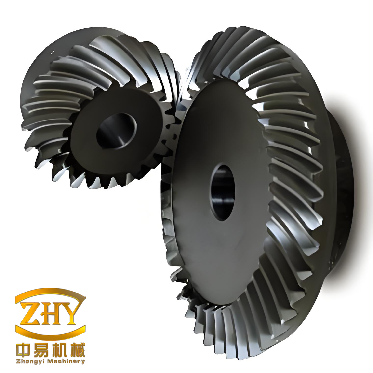
The proposed screw gears are especially attractive for robotic joint reducers because they combine the self-locking tendency, compactness, and high reduction ratio of worm gearing with the internal meshing advantages of internal gear pairs. The internal helical planar enveloping worm drive can be understood as a conjugate pair in which the worm is the generated member and the internal helical gear supplies the generating planar surfaces. The main design variables are the middle-plane module \(m_t\), the base circle radius \(r_b\), the generating plane inclination angle \(\beta\), and the center distance \(A\). These variables control the contact line distribution, lubrication angle, entrainment velocity, and induced normal curvature. I treat these variables as the core of both the performance study and the optimization model.
Geometric and kinematic formulation
I use the moving frame method and differential geometry to describe the conjugate motion of the proposed screw gears. The fixed frames are \(\sigma^{(m)}\) and \(\sigma^{(n)}\), where the worm axis is along \(z_m\) and the internal gear axis is along \(z_n\). The two axes are perpendicular and separated by the center distance \(A\). The rotating frames are \(\sigma^{(1)}\), \(\sigma^{(2)}\), and \(\sigma^{(3)}\). For the forward rotation, I define the angles as
$$
\varphi_1=\omega_1 t,\qquad
\varphi_2=\omega_2 t,\qquad
\varphi_3=2\pi-\theta_0+\varphi_2 .
$$
For the reverse rotation, the worm rotates in the opposite direction, and the corresponding angle relation is
$$
\varphi_2=\omega_2 t,\qquad
\varphi_3=2\pi-\theta_0+\varphi_2,\qquad
\varphi_1’=\frac{1}{i_{12}}\bigl(2\pi-\theta_0-\varphi_2\bigr).
$$
Here \(i_{12}=\omega_1/\omega_2\) is the transmission ratio. The internal helical gear tooth surfaces are planar. In the middle plane, the two sides of the internal gear tooth are tangent to the same base circle. Let \(A\) be the tangent point of the active plane and the base circle, and let \(B\) be the intersection of the same plane with the reference circle. The geometric relations are
$$
\theta_2=\arccos\frac{r_b}{r_2},\qquad
\theta_3=\arccos\frac{r_b}{r_a},\qquad
\tau=\frac{2\pi}{z_2},\qquad
\tau_s=0.55\tau .
$$
Where \(r_2\) is the reference radius, \(r_a\) is the tip radius, \(z_2\) is the number of internal gear teeth, and \(\tau_s\) is the tooth-thickness central angle. The coordinate transformations among the frames are obtained by successive rotations. For the active side, the transformation from \(\sigma^{(1)}\) to the fixed frame \(\sigma^{(m)}\) is
$$
\begin{bmatrix}
\mathbf{i}_1\\ \mathbf{j}_1\\ \mathbf{k}_1
\end{bmatrix}
=
\begin{bmatrix}
\cos\varphi_1 & \sin\varphi_1 & 0\\
-\sin\varphi_1 & \cos\varphi_1 & 0\\
0&0&1
\end{bmatrix}
\begin{bmatrix}
\mathbf{i}_m\\ \mathbf{j}_m\\ \mathbf{k}_m
\end{bmatrix}.
$$
For the generated side, the transformation from \(\sigma^{(2)}\) to the fixed frame \(\sigma^{(n)}\) is
$$
\begin{bmatrix}
\mathbf{i}_2\\ \mathbf{j}_2\\ \mathbf{k}_2
\end{bmatrix}
=
\begin{bmatrix}
\cos\varphi_2 & -\sin\varphi_2 & 0\\
\sin\varphi_2 & \cos\varphi_2 & 0\\
0&0&1
\end{bmatrix}
\begin{bmatrix}
\mathbf{i}_n\\ \mathbf{j}_n\\ \mathbf{k}_n
\end{bmatrix}.
$$
The working frame \(\sigma^{(p)}\) is attached to the active planar surface. Its origin is at the intersection of the base circle and the corresponding axis, and the plane inclination angle \(\beta\) defines the orientation of the generating plane. For a point on the active surface, I write the local coordinates as \((u_3,v_3,0)\). The corresponding coordinates in the gear frame are
$$
x_3=v_3\sin\beta+r_b,\qquad
y_3=u_3,\qquad
z_3=v_3\cos\beta .
$$
Similarly, for the reverse side, the working frame \(\sigma^{(q)}\) gives
$$
x_2=v_2\sin\beta+r_b,\qquad
y_2=u_2,\qquad
z_2=v_2\cos\beta .
$$
These relations are the basis for the subsequent derivation of relative velocity, meshing function, and contact line equations. I keep the notation general so that the same formulation applies to both the forward and reverse meshing sides of the proposed screw gears.
Meshing functions and contact line equations
The relative velocity between the worm and the internal gear at a contact point is the key quantity. For the active side, the relative velocity in the working frame is obtained by transforming the velocity components from the fixed frame. I denote the relative velocity by \(\mathbf{v}^{(31)}\). Its components in the working frame are
$$
\mathbf{v}^{(31)}=v_x^{(31)}\mathbf{i}_3+v_y^{(31)}\mathbf{j}_3+v_z^{(31)}\mathbf{k}_3 ,
$$
$$
v_x^{(31)}=\omega_1\bigl[(\sin\delta_3)u_3+\cos\delta_3\sin\beta\cos\varphi_3\bigr] ,
$$
$$
v_y^{(31)}=\omega_1\bigl[(\sin\delta_3)(v_3\sin\beta+r_b)\cos\varphi_3-\cos\delta_3\cos\beta\sin\varphi_3\bigr] ,
$$
$$
v_z^{(31)}=\omega_1\bigl[(v_3\sin\beta+r_b)\cos\delta_3\cos\varphi_3+\cos\delta_3\sin\beta\sin\varphi_3\bigr] .
$$
The normal vector of the active plane is \(\mathbf{n}^{(3)}=\mathbf{x}_p\). In the working frame, it can be expressed as
$$
\mathbf{n}^{(3)}=\cos\beta\,\mathbf{i}_3+\sin\beta\,\mathbf{k}_3 .
$$
The meshing function is the scalar product of the normal vector and the relative velocity:
$$
\Phi^{(3)}=\mathbf{n}^{(3)}\cdot\mathbf{v}^{(31)}=0 .
$$
Substituting the velocity components and the normal vector yields the explicit meshing function
$$
\Phi^{(3)}=\omega_1\Bigl[
(\sin\delta_3)u_3\cos\beta
+\cos\delta_3\sin\beta\cos\varphi_3\cos\beta
+\cos\delta_3\sin\beta\sin\varphi_3\sin\beta
\Bigr]=0 .
$$
Solving this equation for \(v_3\) gives the contact line equation on the active side:
$$
v_3=u_3\tan\beta
+\frac{A}{\sin\beta\cos\varphi_3}
+\frac{r_b\cos\delta_3}{\sin\beta}
-\frac{\cos\delta_3\sin\varphi_3}{\cos\beta} .
$$
For the reverse side, the same procedure gives the meshing function
$$
\Phi^{(2)}=\mathbf{n}^{(2)}\cdot\mathbf{v}^{(21)}=0 ,
$$
and the corresponding contact line equation
$$
v_2=u_2\tan\beta
+\frac{A}{\sin\beta\cos\varphi_2}
+\frac{r_b\cos\delta_2}{\sin\beta}
-\frac{\cos\delta_2\sin\varphi_2}{\cos\beta} .
$$
These equations show that the contact lines of the proposed screw gears are straight lines in the generating plane. Their positions and orientations are controlled by the module, base circle radius, inclination angle, and center distance. The contact lines are not arbitrary; they must remain inside the effective tooth surface region. The boundary conditions are
$$
u_{\min}=0.5\bigl(m_t z_2-2h_a^*m_t\bigr),\qquad
u_{\max}=0.5\bigl(m_t z_2+2h_f^*m_t\bigr),
$$
$$
u_d=r_b-\sqrt{r_a^2-r_b^2},\qquad
u_u=r_b-\sqrt{r_f^2-r_b^2}.
$$
Where \(h_a^*\) is the addendum coefficient, \(h_f^*\) is the dedendum coefficient, \(r_a\) is the tip radius, and \(r_f\) is the root radius. The contact line range is therefore \(u_d\le u_3\le u_u\) and \(v_{\min}\le v_3\le v_{\max}\).
Boundary curves
The boundary curves of the proposed screw gears are important because they determine whether the contact lines remain within the valid meshing region and whether undercutting occurs. The second kind of boundary curve is obtained by the condition
$$
\Phi^{(3)}=0,\qquad \Phi_t^{(3)}=\frac{\partial \Phi^{(3)}}{\partial t}=0 .
$$
This curve is the envelope of the contact lines on the generating plane. It divides the plane into a meshing region and a non-meshing region. Points inside the meshing region participate in two meshing events, while points on the boundary curve participate only once. For the active side, the second boundary curve is
$$
\Phi_t^{(3)}=\omega_1\Bigl[
\cos\delta_3\cos\varphi_3\cos\beta
-\sin\delta_3\sin\varphi_3\cos\beta
-\sin\delta_3\cos\beta
\Bigr]=0 .
$$
The first kind of boundary curve is obtained by combining the meshing function with the equation of the contact line envelope. It represents the undercutting limit and must lie inside the worm root region. For the active side, I write
$$
\Psi^{(3)}=0,\qquad \Phi^{(3)}=0 .
$$
The explicit form of \(\Psi^{(3)}\) involves the first and second fundamental quantities of the generated surface. I define
$$
E^{(3)}=\mathbf{r}_u^{(3)}\cdot\mathbf{r}_u^{(3)},\qquad
F^{(3)}=\mathbf{r}_u^{(3)}\cdot\mathbf{r}_v^{(3)},\qquad
G^{(3)}=\mathbf{r}_v^{(3)}\cdot\mathbf{r}_v^{(3)},\qquad
D^{(3)}=E^{(3)}G^{(3)}-\bigl(F^{(3)}\bigr)^2 .
$$
The first boundary function is then expressed as
$$
\Psi^{(3)}=\frac{1}{D^{(3)}}\Bigl[
G^{(3)}\Phi_u^{(3)}-F^{(3)}\Phi_v^{(3)},\;
F^{(3)}\Phi_u^{(3)}-E^{(3)}\Phi_v^{(3)}
\Bigr]\cdot
\Bigl[
\mathbf{r}_u^{(3)}\times\mathbf{r}_v^{(3)}
\Bigr] .
$$
These boundary curves are used in the numerical analysis to verify that the contact lines do not cross into the invalid region. I also use them to guide the selection of the optimization constraints.
Lubrication angle, entrainment velocity, and induced normal curvature
For the proposed screw gears, the macro-scale performance is governed by the contact line distribution, while the micro-scale performance is governed by the lubrication angle, entrainment velocity, and induced normal curvature. I define the normal line vector on the contact line as \(\boldsymbol{\sigma}^{(i)}\). It is perpendicular to the common tangent plane of the conjugate surfaces. For the active side, the components are
$$
\sigma_x^{(3)}=\omega_1\sin\delta_3\sin\varphi_3\cos\beta ,
$$
$$
\sigma_y^{(3)}=\omega_1\bigl[(\sin\delta_3)\cos\beta+\sin\beta\cos\varphi_3\cos\delta_3\bigr] ,
$$
$$
\sigma_z^{(3)}=\omega_1\cos\delta_3\sin\varphi_3\cos\beta .
$$
The square of the normal line vector is
$$
\bigl|\boldsymbol{\sigma}^{(3)}\bigr|^2
=\omega_1^2\Bigl[
\cos^2\delta_3\sin^2\varphi_3\cos^2\beta
+\bigl((\sin\delta_3)\cos\beta+\sin\beta\cos\varphi_3\cos\delta_3\bigr)^2
+\cos^2\delta_3\sin^2\varphi_3\cos^2\beta
\Bigr] .
$$
The lubrication angle \(\theta_\tau^{(3)}\) is the acute angle between the contact line tangent direction and the relative velocity projected onto the common tangent plane. It is calculated from
$$
\theta_\tau^{(3)}=\arcsin\left(
\frac{\boldsymbol{\sigma}^{(3)}\cdot\mathbf{v}^{(31)}}
{\bigl|\boldsymbol{\sigma}^{(3)}\bigr|\,\bigl|\mathbf{v}^{(31)}\bigr|}
\right).
$$
A lubrication angle close to \(90^\circ\) is desirable because it promotes the formation of a hydrodynamic oil film and reduces metal-to-metal contact. The entrainment velocity is defined as half of the sum of the two surface velocities along the normal direction:
$$
v_\sigma^{(3)}=\frac{1}{2}
\frac{\boldsymbol{\sigma}^{(3)}\cdot\mathbf{v}^{(31)}}
{\bigl|\boldsymbol{\sigma}^{(3)}\bigr|} .
$$
A larger entrainment velocity helps to build a thicker lubricant film and reduces the risk of scuffing. The induced normal curvature is
$$
k_\sigma^{(31)}=\frac{\Psi^{(3)}}{\bigl|\boldsymbol{\sigma}^{(3)}\bigr|^2} .
$$
A smaller absolute induced normal curvature means that the two conjugate surfaces are more conformal along the contact direction. This reduces contact stress and improves load capacity. The same formulas apply to the reverse side with the corresponding superscripts.
Numerical model and baseline parameters
I use the baseline parameters listed in Table 1 for the numerical study. These parameters are selected according to common design practice and are used as the starting point for the optimization.
| Parameter | Symbol | Value | Unit |
|---|---|---|---|
| Middle-plane module | \(m_t\) | 4 | mm |
| Base circle radius | \(r_b\) | 62.5 | mm |
| Generating plane inclination | \(\beta\) | 19.5 | deg |
| Center distance | \(A\) | 100 | mm |
| Number of worm starts | \(z_1\) | 1 | — |
| Number of internal gear teeth | \(z_2\) | 80 | — |
| Number of simultaneously meshing teeth | \(z’\) | 4 | — |
| Face width | \(B\) | 110 | mm |
The working angle of the internal gear is
$$
\varphi_{2w}=\arcsin\frac{r_b}{r_2},\qquad
\varphi_0=\frac{1}{2}\bigl(\varphi_{2w}+0.45\tau\bigr),\qquad
\varphi’=\varphi_0+\varphi_{2w}.
$$
For each meshing tooth pair, the rotation angle of the working frame is
$$
\varphi_i(j)=\varphi_0-(j-1)\tau,\qquad
j=1,2,\dots,z’+1 .
$$
The analysis angle is defined as
$$
\delta_0=\varphi_0-(n-1)\tau,\qquad
\delta_s=\delta_0-(n-1)\tau .
$$
These definitions allow me to sample the contact lines at equal angular intervals and to evaluate the meshing parameters along each contact line.
Influence of design parameters on contact line distribution
I first study the macro-scale contact behavior. The contact area \(S_p\) and the mean-square end distances \(E_a\) and \(E_b\) are used to quantify the contact line distribution. They are defined as
$$
E_a=\frac{1}{z’}\sum_{j=1}^{z’}\bigl(v_{a(j+1)}-v_{aj}\bigr)^2,\qquad
E_b=\frac{1}{z’}\sum_{j=1}^{z’}\bigl(v_{b(j+1)}-v_{bj}\bigr)^2,
$$
$$
S_p=\frac{1}{2}\Bigl[
\max(v_a)-\min(v_a)+\max(v_b)-\min(v_b)
\Bigr]\bigl(u_u-u_d\bigr).
$$
A larger contact area and larger end-distance mean squares indicate a more uniform contact line distribution and better utilization of the tooth surface. I vary one parameter at a time while keeping the other baseline parameters unchanged. Table 2 summarizes the influence of the middle-plane module on the contact line distribution.
| \(m_t\) (mm) | \(E_a\) (mm\(^2\)) | \(E_b\) (mm\(^2\)) | \(S_p\) (mm\(^2\)) | Observation |
|---|---|---|---|---|
| 3.7 | 12.81 | 12.25 | 90.34 | Contact lines are relatively concentrated. |
| 4.0 | 15.19 | 14.52 | 104.36 | Baseline distribution. |
| 4.2 | 17.07 | 16.34 | 115.01 | Contact area increases. |
| 4.5 | 20.49 | 19.61 | 133.26 | Most dispersed distribution. |
The results show that increasing the module expands the contact area and spreads the contact lines. This improves the load-sharing behavior of the proposed screw gears. However, a larger module also increases the overall size, so it must be balanced against the packaging constraints.
Table 3 shows the influence of the base circle radius on the contact line distribution. As \(r_b\) increases, the pressure angle increases and the contact area tends to decrease. The contact lines become more concentrated, which reduces the effective utilization of the tooth surface.
| \(r_b\) (mm) | \(E_a\) (mm\(^2\)) | \(E_b\) (mm\(^2\)) | \(S_p\) (mm\(^2\)) | Observation |
|---|---|---|---|---|
| 55.5 | 18.05 | 17.16 | 111.13 | Wide distribution, lower pressure angle. |
| 59.0 | 16.41 | 15.71 | 107.19 | Slightly more concentrated. |
| 62.5 | 15.19 | 14.52 | 115.01 | Baseline. |
| 66.0 | 14.28 | 13.63 | 102.46 | Most concentrated. |
Table 4 shows the influence of the generating plane inclination angle. Increasing \(\beta\) shifts the contact lines to the right, enlarges the contact area, and increases the end-distance mean squares. The contact lines become more dispersed, which is generally beneficial for load capacity and thermal behavior.
| \(\beta\) (deg) | \(E_a\) (mm\(^2\)) | \(E_b\) (mm\(^2\)) | \(S_p\) (mm\(^2\)) | Observation |
|---|---|---|---|---|
| 17.0 | 8.89 | 8.97 | 81.22 | Narrow contact region. |
| 18.0 | 12.88 | 12.52 | 96.70 | Moderate expansion. |
| 19.5 | 15.19 | 14.52 | 104.36 | Baseline. |
| 21.0 | 23.42 | 21.58 | 127.50 | Strong expansion and dispersion. |
Table 5 shows the influence of the center distance. As \(A\) increases, the contact lines shift to the left, the contact area increases, and the end-distance mean squares increase. This indicates that a larger center distance can improve the contact line distribution, but it also increases the overall size and may reduce the entrainment velocity.
| \(A\) (mm) | \(E_a\) (mm\(^2\)) | \(E_b\) (mm\(^2\)) | \(S_p\) (mm\(^2\)) | Observation |
|---|---|---|---|---|
| 60 | 10.13 | 9.58 | 85.10 | Compact but concentrated. |
| 80 | 12.54 | 11.86 | 94.76 | Moderate distribution. |
| 100 | 15.19 | 14.52 | 104.36 | Baseline. |
| 120 | 18.11 | 17.53 | 113.06 | Wide distribution but larger envelope. |
Influence of design parameters on lubrication angle
The lubrication angle is one of the most important micro-scale indicators for the proposed screw gears. I calculate it at five equally spaced points on each contact line. Table 6 shows the baseline lubrication angle distribution for the active side. The lubrication angle decreases from the meshing-in end to the meshing-out end, and it increases toward the root direction along the same contact line.
| \(\varphi_3\) (deg) | \(u=u_1\) | \(u=u_2\) | \(u=u_3\) | \(u=u_4\) | \(u=u_5\) |
|---|---|---|---|---|---|
| 28.5059 | 86.8678 | 87.2169 | 87.4961 | 87.7244 | 87.9145 |
| 24.0059 | 86.3093 | 86.7340 | 87.0712 | 87.3453 | 87.5725 |
| 19.5059 | 85.4145 | 85.9635 | 86.3953 | 86.7437 | 87.0308 |
| 15.0059 | 83.8779 | 84.6462 | 85.2435 | 85.7211 | 86.1117 |
Table 7 summarizes the effect of the module on the lubrication angle. A larger module increases the lubrication angle and improves the lubrication condition. This is beneficial for the formation of a hydrodynamic film in the proposed screw gears.
| \(m_t\) (mm) | \(\delta_1\) | \(\delta_2\) | \(\delta_3\) | \(\delta_4\) | Average trend |
|---|---|---|---|---|---|
| 3.7 | 86.25 | 85.63 | 84.64 | 82.99 | Lowest |
| 4.0 | 86.87 | 86.31 | 85.41 | 83.88 | Baseline |
| 4.2 | 87.15 | 86.62 | 85.75 | 84.24 | Improved |
| 4.5 | 87.46 | 86.95 | 86.11 | 84.59 | Highest |
Table 8 shows the effect of the base circle radius. Increasing \(r_b\) also increases the lubrication angle, but the effect is weaker than that of the module. The lubrication performance improves slightly as the base circle radius grows.
| \(r_b\) (mm) | \(\delta_1\) | \(\delta_2\) | \(\delta_3\) | \(\delta_4\) | Average trend |
|---|---|---|---|---|---|
| 55.5 | 86.57 | 85.88 | 84.73 | 82.63 | Lowest |
| 59.0 | 86.72 | 86.11 | 85.10 | 83.31 | Improved |
| 62.5 | 86.87 | 86.31 | 85.41 | 83.88 | Baseline |
| 66.0 | 87.00 | 86.49 | 85.69 | 84.35 | Highest |
Table 9 shows the effect of the generating plane inclination angle. The influence of \(\beta\) on the lubrication angle is small. The lubrication angle changes only slightly when \(\beta\) is varied, so this parameter can be given a lower weight in the optimization objective.
| \(\beta\) (deg) | \(\delta_1\) | \(\delta_2\) | \(\delta_3\) | \(\delta_4\) | Average trend |
|---|---|---|---|---|---|
| 18.0 | 86.92 | 86.38 | 85.51 | 84.03 | Slightly higher |
| 19.0 | 86.89 | 86.34 | 85.46 | 83.93 | Close to baseline |
| 19.5 | 86.87 | 86.31 | 85.41 | 83.88 | Baseline |
| 21.0 | 86.86 | 86.31 | 85.46 | 84.07 | Nearly unchanged |
Table 10 shows the effect of the center distance. The lubrication angle decreases significantly as the center distance increases. A smaller center distance is therefore favorable for lubrication, but it may reduce the contact area and the entrainment velocity. This trade-off must be handled by the optimization model.
| \(A\) (mm) | \(\delta_1\) | \(\delta_2\) | \(\delta_3\) | \(\delta_4\) | Average trend |
|---|---|---|---|---|---|
| 60 | 88.97 | 88.79 | 88.51 | 88.05 | Highest |
| 80 | 88.23 | 87.92 | 87.43 | 86.60 | High |
| 100 | 86.87 | 86.31 | 85.41 | 83.88 | Baseline |
| 120 | 83.59 | 82.42 | 80.46 | 76.97 | Lowest |
Influence of design parameters on entrainment velocity
The entrainment velocity is another important micro-scale indicator. I evaluate it at the same five points on each contact line. Table 11 shows the baseline entrainment velocity for the active side. The entrainment velocity first increases and then decreases as the working angle changes. Along a single contact line, it increases with \(u\).
| \(\varphi_3\) (deg) | \(u=u_1\) | \(u=u_2\) | \(u=u_3\) | \(u=u_4\) | \(u=u_5\) |
|---|---|---|---|---|---|
| 28.5059 | 3.0763 | 3.4567 | 3.8371 | 4.2174 | 4.5978 |
| 24.0059 | 3.0635 | 3.4565 | 3.8495 | 4.2425 | 4.6355 |
| 19.5059 | 3.0046 | 3.4081 | 3.8117 | 4.2153 | 4.6189 |
| 15.0059 | 2.9003 | 3.3123 | 3.7244 | 4.1365 | 4.5485 |
Table 12 shows the effect of the module on the entrainment velocity. A larger module significantly increases the entrainment velocity. This is favorable for oil film formation and for reducing friction and wear in the proposed screw gears.
| \(m_t\) (mm) | \(\delta_1\) | \(\delta_2\) | \(\delta_3\) | \(\delta_4\) | Average trend |
|---|---|---|---|---|---|
| 3.7 | 2.43 | 2.41 | 2.35 | 2.25 | Lowest |
| 4.0 | 3.08 | 3.06 | 3.00 | 2.90 | Baseline |
| 4.2 | 3.51 | 3.49 | 3.44 | 3.33 | Improved |
| 4.5 | 4.14 | 4.14 | 4.08 | 3.96 | Highest |
Table 13 shows the effect of the base circle radius. The entrainment velocity is almost independent of \(r_b\). The changes are very small, so the base circle radius mainly affects the contact geometry and the pressure angle rather than the entrainment velocity.
| \(r_b\) (mm) | \(\delta_1\) | \(\delta_2\) | \(\delta_3\) | \(\delta_4\) | Average trend |
|---|---|---|---|---|---|
| 55.5 | 3.078 | 3.071 | 3.018 | 2.921 | Nearly constant |
| 59.0 | 3.077 | 3.067 | 3.011 | 2.911 | Nearly constant |
| 62.5 | 3.076 | 3.064 | 3.005 | 2.900 | Baseline |
| 66.0 | 3.075 | 3.059 | 2.997 | 2.890 | Nearly constant |
Table 14 shows the effect of the generating plane inclination angle. The entrainment velocity is not strongly affected by \(\beta\). The variations are small, so this parameter can be assigned a lower weight in the optimization.
| \(\beta\) (deg) | \(\delta_1\) | \(\delta_2\) | \(\delta_3\) | \(\delta_4\) | Average trend |
|---|---|---|---|---|---|
| 18.0 | 3.094 | 3.085 | 3.028 | 2.920 | Nearly constant |
| 19.0 | 3.085 | 3.073 | 3.013 | 2.903 | Nearly constant |
| 19.5 | 3.076 | 3.064 | 3.005 | 2.900 | Baseline |
| 21.0 | 3.075 | 3.069 | 3.027 | 2.959 | Nearly constant |
Table 15 shows the effect of the center distance. The entrainment velocity decreases strongly as \(A\) increases. A smaller center distance produces a higher entrainment velocity, which is favorable for lubrication. However, a smaller center distance also reduces the contact area and may increase the pressure angle. This trade-off is addressed in the optimization.
| \(A\) (mm) | \(\delta_1\) | \(\delta_2\) | \(\delta_3\) | \(\delta_4\) | Average trend |
|---|---|---|---|---|---|
| 60 | 5.567 | 5.562 | 5.509 | 5.409 | Highest |
| 80 | 4.322 | 4.313 | 4.257 | 4.155 | High |
| 100 | 3.076 | 3.064 | 3.005 | 2.900 | Baseline |
| 120 | 1.831 | 1.815 | 1.753 | 1.646 | Lowest |
Influence of design parameters on induced normal curvature
The induced normal curvature is a measure of the conformity of the conjugate surfaces. A smaller absolute value is preferred. Table 16 shows the baseline induced normal curvature for the active side. The induced normal curvature decreases as the working angle decreases and as \(u\) increases.
| \(\varphi_3\) (deg) | \(u=u_1\) | \(u=u_2\) | \(u=u_3\) | \(u=u_4\) | \(u=u_5\) |
|---|---|---|---|---|---|
| 28.5059 | 0.0093 | 0.0083 | 0.0075 | 0.0068 | 0.0062 |
| 24.0059 | 0.0080 | 0.0070 | 0.0063 | 0.0057 | 0.0052 |
| 19.5059 | 0.0066 | 0.0059 | 0.0052 | 0.0047 | 0.0043 |
| 15.0059 | 0.0053 | 0.0047 | 0.0041 | 0.0037 | 0.0034 |
Table 17 shows the effect of the module on the induced normal curvature. Increasing the module reduces the induced normal curvature, which is beneficial for reducing contact stress and improving the load capacity of the proposed screw gears.
| \(m_t\) (mm) | \(\delta_1\) | \(\delta_2\) | \(\delta_3\) | \(\delta_4\) | Average trend |
|---|---|---|---|---|---|
| 3.7 | 0.0126 | 0.0109 | 0.0093 | 0.0078 | Highest |
| 4.0 | 0.0093 | 0.0080 | 0.0066 | 0.0053 | Baseline |
| 4.2 | 0.0079 | 0.0066 | 0.0055 | 0.0043 | Lower |
| 4.5 | 0.0063 | 0.0053 | 0.0042 | 0.0032 | Lowest |
Table 18 shows the effect of the base circle radius. The induced normal curvature increases as \(r_b\) increases. A larger base circle radius therefore reduces the conformity of the conjugate surfaces and may increase contact stress. This is an important trade-off in the optimization.
| \(r_b\) (mm) | \(\delta_1\) | \(\delta_2\) | \(\delta_3\) | \(\delta_4\) | Average trend |
|---|---|---|---|---|---|
| 55.5 | 0.0085 | 0.0071 | 0.0057 | 0.0043 | Lowest |
| 59.0 | 0.0089 | 0.0075 | 0.0062 | 0.0048 | Higher |
| 62.5 | 0.0093 | 0.0080 | 0.0066 | 0.0053 | Baseline |
| 66.0 | 0.0097 | 0.0084 | 0.0071 | 0.0058 | Highest |
Table 19 shows the effect of the generating plane inclination angle. The induced normal curvature changes only slightly with \(\beta\). The effect is small, so this parameter can be given a lower weight in the optimization.
| \(\beta\) (deg) | \(\delta_1\) | \(\delta_2\) | \(\delta_3\) | \(\delta_4\) | Average trend |
|---|---|---|---|---|---|
| 18.0 | 0.0094 | 0.0080 | 0.0067 | 0.0054 | Slightly higher |
| 19.0 | 0.0093 | 0.0080 | 0.0067 | 0.0054 | Close to baseline |
| 19.5 | 0.0093 | 0.0080 | 0.0066 | 0.0053 | Baseline |
| 21.0 | 0.0093 | 0.0079 | 0.0066 | 0.0052 | Nearly unchanged |
Table 20 shows the effect of the center distance. The induced normal curvature increases significantly as \(A\) increases. A larger center distance reduces the conformity of the conjugate surfaces and increases contact stress. This is consistent with the trend observed for the entrainment velocity and lubrication angle. The optimization must therefore find a balanced center distance that satisfies all performance requirements.
| \(A\) (mm) | \(\delta_1\) | \(\delta_2\) | \(\delta_3\) | \(\delta_4\) | Average trend |
|---|---|---|---|---|---|
| 60 | 0.0051 | 0.0044 | 0.0036 | 0.0028 | Lowest |
| 80 | 0.0066 | 0.0056 | 0.0047 | 0.0037 | Higher |
| 100 | 0.0093 | 0.0080 | 0.0066 | 0.0053 | Baseline |
| 120 | 0.0158 | 0.0135 | 0.0115 | 0.0094 | Highest |
Optimization model for the proposed screw gears
Based on the parametric study, I formulate a multi-objective nonlinear optimization problem for the proposed screw gears. The design variables are
$$
\mathbf{x}=[m_t,\;r_b,\;\beta,\;A].
$$
The optimization aims to improve both the macro-scale and micro-scale meshing performance. The macro-scale objective is to enlarge the contact area and to spread the contact lines uniformly. The micro-scale objective is to increase the lubrication angle, increase the entrainment velocity, and reduce the absolute induced normal curvature. I define the sub-objectives as follows:
$$
\min f_1(\mathbf{x})=\frac{1}{S_p},
$$
$$
\min f_2(\mathbf{x})=\frac{1}{E_a+E_b},
$$
$$
\min f_3(\mathbf{x})=\frac{1}{\overline{\theta}_\tau},
$$
$$
\min f_4(\mathbf{x})=\frac{1}{\overline{v}_\sigma},
$$
$$
\min f_5(\mathbf{x})=\overline{|k_\sigma|}.
$$
The averaged quantities are defined over all sampled meshing points on the active side:
$$
\overline{\theta}_\tau=
\frac{1}{z’}\sum_{j=1}^{z’}\sum_{m=1}^{5}
\theta_\tau^{(3)}\bigl(u(m),\varphi_3(j)\bigr),
$$
$$
\overline{v}_\sigma=
\frac{1}{z’}\sum_{j=1}^{z’}\sum_{m=1}^{5}
v_\sigma^{(3)}\bigl(u(m),\varphi_3(j)\bigr),
$$
$$
\overline{|k_\sigma|}=
\frac{1}{z’}\sum_{j=1}^{z’}\sum_{m=1}^{5}
\bigl|k_\sigma^{(31)}\bigl(u(m),\varphi_3(j)\bigr)\bigr|.
$$
I normalize each sub-objective by its independently optimized minimum:
$$
F_i(\mathbf{x})=\frac{f_i(\mathbf{x})}{\min f_i(\mathbf{x})},\qquad i=1,2,\dots,5.
$$
The overall objective is a weighted combination of the normalized sub-objectives:
$$
\min F(\mathbf{x})=
0.25F_1+0.25F_2+0.15F_3+0.20F_4+0.15F_5.
$$
The constraints are chosen to ensure a valid and manufacturable design. The pressure angle must remain between \(20^\circ\) and \(25^\circ\):
$$
20^\circ\le \alpha\le 25^\circ,
\qquad
\alpha=\arcsin\frac{r_b}{r_2}.
$$
The contact lines must lie inside the effective tooth surface:
$$
\max(v_a)-u_u\le 0,\qquad
\min(v_a)-u_d\ge 0,
$$
$$
\max(v_b)-u_u\le 0,\qquad
\min(v_b)-u_d\ge 0.
$$
The sliding velocity must not exceed the allowable limit:
$$
V_h\le 12\ \text{m/s}.
$$
The bounds of the design variables are
$$
3.69\le m_t\le 4.93,\qquad
54.72\le r_b\le 67.62,
$$
$$
0^\circ\le \beta\le 20.34^\circ,\qquad
60\le A\le 120.
$$
I solve the optimization problem with the sequential quadratic programming algorithm implemented in the fmincon function. The initial point is the baseline design:
$$
\mathbf{x}_0=[4,\;62.5,\;19.5,\;100].
$$
The optimized design variables are
$$
\mathbf{x}^*=[5.09,\;69.59,\;21.99,\;88.86].
$$
Table 21 compares the optimization variables and their bounds. The optimized module is larger than the baseline, the base circle radius is larger, the inclination angle is slightly larger, and the center distance is smaller. These changes are consistent with the parametric trends observed in the previous section.
| Variable | Lower bound | Upper bound | Initial value | Optimized value |
|---|---|---|---|---|
| \(m_t\) (mm) | 3.69 | 4.93 | 4.00 | 5.09 |
| \(r_b\) (mm) | 54.72 | 67.62 | 62.50 | 69.59 |
| \(\beta\) (deg) | 0 | 20.34 | 19.50 | 21.99 |
| \(A\) (mm) | 60 | 120 | 100 | 88.86 |
The optimization improves the contact line distribution and the micro-scale meshing parameters. Table 22 compares the lubrication angle before and after optimization. The average lubrication angle increases, and the improvement is consistent across all sampled positions.
| \(\varphi_3\) (deg) | Before optimization | After optimization | Improvement (%) |
|---|---|---|---|
| \(\delta_1\) | 87.91 | 88.54 | 0.72 |
| \(\delta_2\) | 87.57 | 88.26 | 0.79 |
| \(\delta_3\) | 87.03 | 87.80 | 0.89 |
| \(\delta_4\) | 86.11 | 87.00 | 1.03 |
Table 23 compares the entrainment velocity before and after optimization. The entrainment velocity increases by about \(58.8\%\), which is a substantial improvement for oil film formation and scuffing resistance in the proposed screw gears.
| \(\varphi_3\) (deg) | Before optimization (mm/s) | After optimization (mm/s) | Improvement (%) |
|---|---|---|---|
| \(\delta_1\) | 4.60 | 7.25 | 57.61 |
| \(\delta_2\) | 4.55 | 7.31 | 60.66 |
| \(\delta_3\) | 4.62 | 7.30 | 58.01 |
| \(\delta_4\) | 4.55 | 7.23 | 58.90 |
Table 24 compares the induced normal curvature before and after optimization. The absolute induced normal curvature decreases by about \(46.32\%\), which indicates better conformity of the conjugate surfaces and lower contact stress.
| \(\varphi_3\) (deg) | Before optimization | After optimization | Reduction (%) |
|---|---|---|---|
| \(\delta_1\) | 0.0062 | 0.0035 | 43.55 |
| \(\delta_2\) | 0.0052 | 0.0029 | 44.23 |
| \(\delta_3\) | 0.0043 | 0.0023 | 46.51 |
| \(\delta_4\) | 0.0034 | 0.0017 | 50.00 |
The optimization results show that the proposed screw gears achieve a better balance between load capacity, lubrication, and surface conformity. The contact area increases, the contact lines become more uniformly distributed, the lubrication angle approaches the ideal value of \(90^\circ\), the entrainment velocity increases substantially, and the induced normal curvature decreases. These improvements are consistent with the theoretical predictions and confirm the effectiveness of the optimization model.
Three-dimensional modeling and virtual assembly
I use the optimized parameters to build a three-dimensional model of the proposed screw gears. The worm tooth surface is complex because its geometry changes continuously along the axial direction. Conventional extrusion, revolution, or sweep commands cannot directly generate the exact tooth surface. I therefore adopt the boundary representation method. The boundary representation method describes the solid by its bounding surfaces, curves, and vertices, and it is well suited to complex worm surfaces.
The modeling procedure consists of five steps. First, I establish the mathematical model of the worm surface and generate the variable-radius helices in a numerical environment. Second, I export the helix data as an .ibl file. Third, I import the file into the three-dimensional modeling environment. Fourth, I use boundary blending to construct the worm tooth surface. Fifth, I merge the surfaces and convert them into a solid model.
The variable-radius helices are obtained from the contact line equations and the meshing functions. For the active side, the helix is parameterized by
$$
\mathbf{r}^{(3)}(u_3,\varphi_3)=
x_3\mathbf{i}_3+y_3\mathbf{j}_3+z_3\mathbf{k}_3,
$$
$$
x_3=v_3\sin\beta+r_b,\qquad
y_3=u_3,\qquad
z_3=v_3\cos\beta,
$$
$$
v_3=u_3\tan\beta
+\frac{A}{\sin\beta\cos\varphi_3}
+\frac{r_b\cos\delta_3}{\sin\beta}
-\frac{\cos\delta_3\sin\varphi_3}{\cos\beta}.
$$
For the reverse side, the same procedure is applied with the corresponding reverse-side parameters. The helix data are written in the .ibl format and imported into the modeling environment. The boundary blending tool then generates a smooth and continuous tooth surface. I repeat this process for both sides of the worm thread and merge the resulting surfaces with the worm body.
After the worm solid is completed, I build the internal helical gear according to the same design parameters. The internal gear is simpler to model because its tooth surfaces are planar. I then assemble the worm and the internal gear in the virtual assembly environment. The assembly constraints are defined by the center distance, the axis orientation, and the meshing phase. I use the static global interference check to verify the assembly. No interference is detected, which confirms that the geometric model is consistent with the theoretical meshing conditions.
The virtual assembly provides a basis for subsequent manufacturing, finite element analysis, and dynamic simulation. It also confirms that the optimized design can be realized as a physical transmission. The proposed screw gears are therefore not only theoretically valid but also geometrically manufacturable.
Summary of contributions
I have developed a complete theoretical and computational framework for internal helical planar enveloping worm drives, which belong to the family of screw gears. The main contributions are as follows. First, I established a moving-frame formulation for both forward and reverse rotations and derived the meshing functions, contact line equations, and boundary curve equations. Second, I derived the lubrication angle, entrainment velocity, and induced normal curvature formulas and used them to evaluate the macro-scale and micro-scale performance. Third, I performed a systematic parametric study and quantified the influence of the module, base circle radius, generating plane inclination angle, and center distance. Fourth, I formulated a multi-objective nonlinear optimization model and solved it with a sequential quadratic programming algorithm. Fifth, I built a three-dimensional model and verified the assembly by interference checking.
The results show that the proposed screw gears can achieve a compact structure, high load capacity, and favorable lubrication performance. The optimized design increases the contact area, improves the contact line distribution, raises the lubrication angle, increases the entrainment velocity, and reduces the induced normal curvature. These improvements are beneficial for robotic joint reducers, precision positioning devices, and other applications that require high reduction ratios and compact envelopes.
Future work
Several directions remain for further study. I plan to extend the model to include thermal effects, elastic deformation, and manufacturing errors. I also intend to build a prototype and conduct break-in tests, transmission accuracy measurements, and efficiency tests. Dynamic simulations with a virtual prototype will be used to evaluate the transient behavior under variable loads and speeds. Finally, I will investigate the integration of the proposed screw gears into a complete robot joint module with an integrated motor, controller, and bearing system. These studies will help to move the internal helical planar enveloping worm drive from a theoretical concept to a practical engineering solution.