
I began this study with a practical question: how can I evaluate and improve the meshing behavior of a hypoid bevel gear used in a vehicle drive axle main reducer? A hypoid bevel gear transmits motion and power between intersecting axes with an offset, and its contact quality, life, and reliability strongly influence vehicle safety. I therefore combined differential geometry, gearing theory, tooth contact analysis, finite element analysis, and tool modification design to study a hypoid bevel gear pair. I used a right-hand gear and a left-hand pinion. The gear was generated by the formate method, and the pinion was generated by the tilt method. I derived the tooth surface equations, performed cutting simulation, built accurate finite element models, studied installation error effects, and optimized curved cutting blades for the pinion. The following sections describe the methods, equations, tables, and results I obtained.
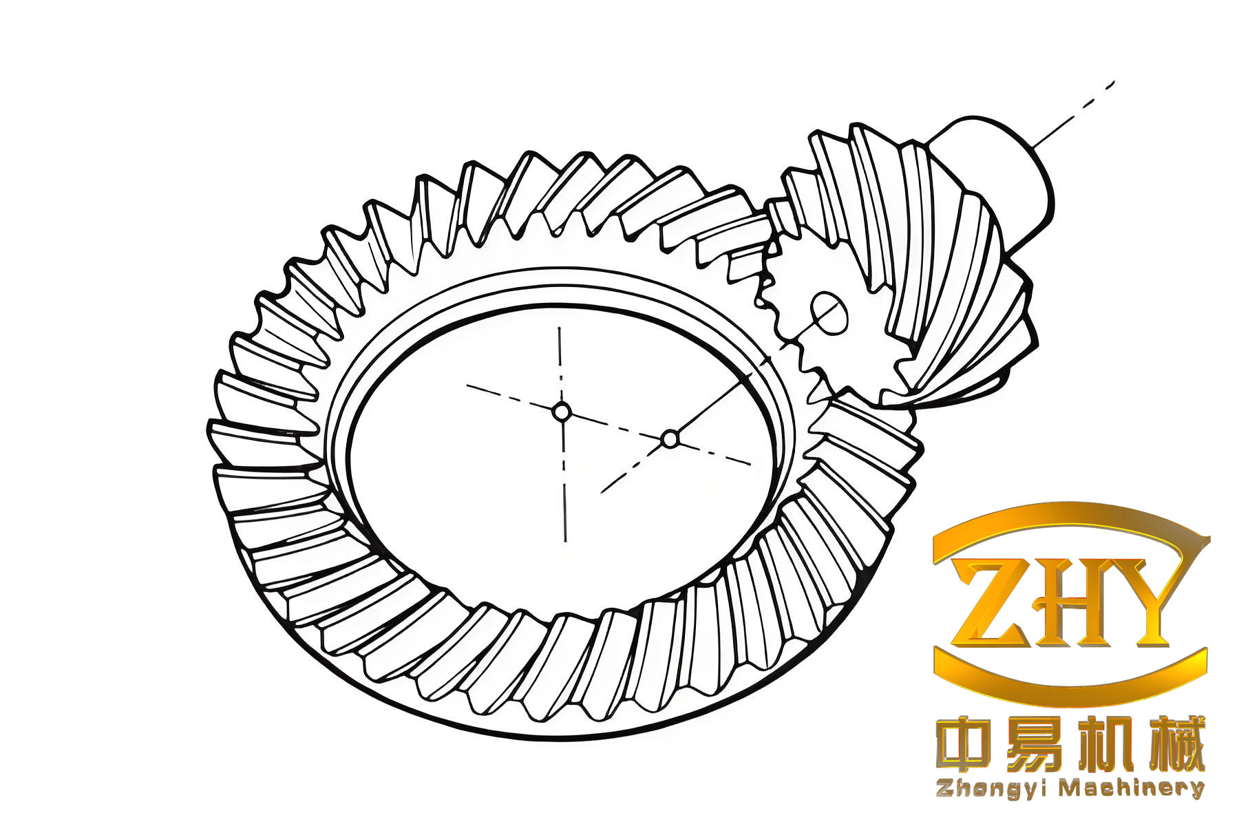
I first established a mathematical model of the hypoid bevel gear tooth surfaces including the transition fillet. For the gear, the cutting tool was a disk with straight edges and a corner radius. I defined the tool coordinate system and the local coordinate system of the transition fillet. The connection point between the straight edge and the fillet satisfied both the position and normal conditions. I wrote the position vector and unit normal vector of the connection point as
$$ r_{02}=[r_f\sin\theta_f,\;0,\;r_f\cos\theta_f]^T $$
$$ n_{02}=[\sin\theta_f,\;0,\;\cos\theta_f]^T $$
where \(r_f\) is the corner radius. For the convex side I used \(\theta_f=\alpha_G\), and for the concave side I used \(\theta_f=\pi-\alpha_G\). The working surface of the gear was expressed in the gear coordinate system as
$$ r_2(s_G,\theta_G)=M_{2B}M_{BG}r_G(s_G,\theta_G) $$
$$ n_2(s_G,\theta_G)=L_{2B}L_{BG}n_G(s_G,\theta_G) $$
where \(s_G\) and \(\theta_G\) are the tool surface parameters, \(M_{2B}\) and \(M_{BG}\) are coordinate transformation matrices, and \(L_{2B}\) and \(L_{BG}\) are the corresponding rotation matrices. The straight cutting edge of the gear tool was written as
$$ r_G(s_G,\theta_G)=\begin{bmatrix} (r_c-s_G\sin\alpha_G)\cos\theta_G \\ (r_c-s_G\sin\alpha_G)\sin\theta_G \\ -s_G\cos\alpha_G \\ 1 \end{bmatrix} $$
$$ n_G(s_G,\theta_G)=\begin{bmatrix} \sin\alpha_G\cos\theta_G \\ \sin\alpha_G\sin\theta_G \\ -\cos\alpha_G \\ 0 \end{bmatrix} $$
The transition surface of the gear was obtained by rotating the fillet profile and transforming it into the gear coordinate system. I wrote it as
$$ r_{2f}(\theta_G,\theta_{2f})=M_{2B}M_{BG}r_{fG}(\theta_G,\theta_{2f}) $$
$$ n_{2f}(\theta_G,\theta_{2f})=L_{2B}L_{BG}n_{fG}(\theta_G,\theta_{2f}) $$
I verified the boundary between the working surface and the transition surface. The coordinates on the boundary from the working surface and from the transition surface were exactly equal. Table 1 shows a representative comparison for the gear flanks.
| Flank | Quantity | Value 1 | Value 2 | Value 3 | Value 4 | Value 5 |
|---|---|---|---|---|---|---|
| Convex | \(h\) from working surface | -3.766 | -4.075 | -4.371 | -4.652 | -4.916 |
| Convex | \(h\) from transition surface | -3.766 | -4.075 | -4.371 | -4.652 | -4.916 |
| Concave | \(h\) from working surface | -3.745 | -4.074 | -4.390 | -4.691 | -4.976 |
| Concave | \(h\) from transition surface | -3.745 | -4.074 | -4.390 | -4.691 | -4.976 |
For the pinion of the hypoid bevel gear, I used the tilt method. The tool coordinate system, the tilt coordinate system, the cradle coordinate system, and the pinion coordinate system were related by a sequence of transformations. The pinion working surface was expressed as
$$ r_1(s_P,\theta_P,\phi_c)=M_{1F}M_{FE}M_{ED}M_{DC}M_{CA}M_{AP}r_P(s_P,\theta_P) $$
$$ n_1(s_P,\theta_P,\phi_c)=L_{1F}L_{FE}L_{ED}L_{DC}L_{CA}L_{AP}n_P(s_P,\theta_P) $$
The meshing equation during pinion generation was
$$ f(s_P,\theta_P,\phi_c)=n_D\cdot v_D^{(c1)}=0 $$
where \(v_D^{(c1)}\) is the relative velocity between the cutter and the pinion blank. Expanding this equation gave
$$ s_P=s_P(\theta_P,\phi_c) $$
Substituting this relation into the pinion surface equations eliminated one parameter and produced the final pinion tooth surface. The pinion transition surface was derived in the same way.
To visualize the tooth surfaces and to prepare for finite element analysis, I divided the working surface and the transition surface into grids on the rotation projection plane. Along the tooth length I used \(n\) columns, and along the tooth height I used \(m\) rows. The coordinates of a grid point were
$$ v_{ij}=A_i+\frac{(j-1)(A_o-A_i)}{n-1},\quad i=1,\ldots,m,\; j=1,\ldots,n $$
$$ h_{ij}=H_j+\frac{(i-1)(h’_j-H_j)}{m-1} $$
where \(A_i\) is the inner cone distance, \(A_o\) is the outer cone distance, \(H_j\) is the top land coordinate, and \(h’_j\) is the boundary coordinate. I solved the nonlinear equations for each grid point and obtained the three-dimensional coordinates of the hypoid bevel gear tooth surfaces. Table 2 lists the basic parameters of the hypoid bevel gear pair I used in my example.
| Parameter | Pinion | Gear |
|---|---|---|
| Number of teeth | 8 | 41 |
| Face width (mm) | 28.09 | 24.00 |
| Outer cone distance (mm) | 97.19 | 84.72 |
| Addendum (mm) | 5.77 | 1.02 |
| Dedendum (mm) | 2.04 | 6.64 |
| Offset (mm) | 23 | |
| Pitch cone angle | \(12^\circ32’\) | \(76^\circ49’\) |
| Face cone angle | \(17^\circ27’\) | \(77^\circ44’\) |
| Root cone angle | \(11^\circ40’\) | \(71^\circ41’\) |
| Spiral angle | \(48^\circ56’\) | \(30^\circ38’\) |
| Tool corner radius (mm) | 0.65 | 1.0 |
| Midpoint chordal height (mm) | 4.80 | 0.83 |
| Midpoint chordal thickness (mm) | 6.12 | 3.09 |
| Hand | LH | RH |
Table 3 gives the gear machine settings, and Table 4 gives the pinion machine settings for the concave and convex sides.
| Gear machine setting | Value |
|---|---|
| Cutter diameter (mm) | 152.40 |
| Point width (mm) | 1.59 |
| Profile angle (degree) | 22.5 |
| Vertical cutter position (mm) | 67.7661 |
| Horizontal cutter position (mm) | 29.8166 |
| Horizontal wheel position (mm) | 0.5984 |
| Blank mounting angle (degree) | 70.88 |
| Pinion machine setting | Concave side | Convex side |
|---|---|---|
| Cutter diameter (mm) | 161.04 | 149.86 |
| Point width (mm) | 0 | 0 |
| Profile angle (degree) | 20.0 | 25.0 |
| Radial cutter position (mm) | 73.9536 | 72.5171 |
| Tilt angle (degree) | 16.73 | 19.17 |
| Cutter rotation angle (degree) | 346.66 | 337.92 |
| Vertical wheel position (mm) | 19.6316 | 23.0267 |
| Horizontal wheel position (mm) | 2.3949 | -1.7553 |
| Sliding base (mm) | 2.6682 | 7.7363 |
| Blank mounting angle (degree) | 358.01 | 355.16 |
| Roll ratio | 5.064418 | 4.816942 |
| Angular cutter position (degree) | 83.61 | 77.42 |
I also had to position the pinion concave and convex surfaces precisely. Because the pinion was cut by the single-side method, the two sides did not form a correct tooth unless I rotated one side relative to the other. I used the midpoint chordal height \(h_{m1}\) and the midpoint chordal thickness \(s_{n1}\) as the inspection dimensions. For a point \(O_v\) on the concave side and a point \(O_x\) on the convex side, I solved
$$ d_v=\sqrt{(R_v-L_v)^2+h_{m1}^2} $$
$$ R_v^2+L_v^2=A_m^2+(0.5s_{n1})^2-2A_m(0.5s_{n1})\cos\left(\frac{\pi}{2}-\beta_1\right) $$
and a similar equation with \(\pi/2+\beta_1\) for the convex side. The positioning angle \(\theta_x\) was then obtained from
$$ s_{n1}=\sqrt{(y_x\cos\theta_x-z_x\sin\theta_x-y_v)^2+(y_x\sin\theta_x+z_x\cos\theta_x-z_v)^2} $$
In my example I found \(\theta_x=2.6406^\circ\). I used the concave side as the datum and rotated the convex side by this angle. The resulting pinion tooth was correct and continuous. I then compared two solid modeling methods: cutting simulation and reverse modeling from point clouds. I measured the deviation between the modeled surface and the mathematical point cloud. Table 5 summarizes the deviations on selected points.
| Surface | Method | Deviation 1 (mm) | Deviation 2 (mm) | Deviation 3 (mm) | Deviation 4 (mm) | Deviation 5 (mm) |
|---|---|---|---|---|---|---|
| Gear convex | Cutting simulation | 0.033 | 0.018 | 0.031 | 0.007 | 0.022 |
| Gear convex | Reverse modeling | 0.035 | 0.044 | 0.086 | 0.124 | 0.116 |
| Gear concave | Cutting simulation | 0.036 | 0.026 | 0.024 | 0.049 | 0.065 |
| Gear concave | Reverse modeling | 0.045 | 0.057 | 0.089 | 0.123 | 0.171 |
| Pinion convex | Cutting simulation | 0.016 | 0.021 | 0.000 | 0.024 | 0.012 |
| Pinion convex | Reverse modeling | 0.098 | 0.000 | 0.019 | 0.030 | 0.064 |
| Pinion concave | Cutting simulation | 0.030 | 0.022 | 0.017 | 0.024 | 0.020 |
| Pinion concave | Reverse modeling | 0.096 | 0.062 | 0.069 | 0.066 | 0.116 |
The cutting simulation method gave smaller deviations than reverse modeling for both the gear and the pinion of the hypoid bevel gear. Therefore, I concluded that cutting simulation is more accurate for solid modeling, and it also validates the mathematical model of the hypoid bevel gear.
Next, I studied tooth contact analysis. In theoretical TCA, the two tooth surfaces are in continuous tangency. In a fixed coordinate system, the position vectors and unit normal vectors must be equal at the contact point. I wrote the basic TCA equations as
$$ r_h^{(1)}(\theta_P,\phi_c,\phi_1)=r_h^{(2)}(s_G,\theta_G,\phi_2) $$
$$ n_h^{(1)}(\theta_P,\phi_c,\phi_1)=n_h^{(2)}(s_G,\theta_G,\phi_2) $$
These equations provided five independent scalar equations. I treated the pinion rotation angle \(\phi_1\) as the input and solved for the remaining five unknowns. Repeating this process produced the contact path. To find the initial contact point, I also required that the instantaneous gear ratio equal the nominal gear ratio. The instantaneous ratio was
$$ i(t)=\frac{p_2\cdot (R_2\times n_2)}{p_1\cdot (R_1\times n_1)} $$
where \(p_1=(-1,0,0)\) and \(p_2=(0,0,1)\) for my coordinate system. The transmission error was defined as
$$ \delta\phi_2=\left(\phi_2-\phi_2^{(0)}\right)-\frac{Z_1}{Z_2}\left(\phi_1-\phi_1^{(0)}\right) $$
I also calculated the instantaneous contact ellipse. The semi-major axis \(a\) and semi-minor axis \(b\) were
$$ a=\sqrt{\frac{\epsilon}{A}},\qquad b=\sqrt{\frac{\epsilon}{B}} $$
where \(\epsilon\) is the elastic deformation, usually taken as \(0.00635\) mm, and \(A\) and \(B\) are functions of the principal curvatures and directions. I used
$$ A=\frac{1}{4}\left[K_1-K_2-\sqrt{g_1^2+g_2^2-2g_1g_2\cos 2\alpha_{12}}\right] $$
$$ B=\frac{1}{4}\left[K_1-K_2+\sqrt{g_1^2+g_2^2-2g_1g_2\cos 2\alpha_{12}}\right] $$
where \(K_1=k_f+k_h\), \(K_2=k_s+k_q\), \(g_1=k_f-k_h\), and \(g_2=k_s-k_q\). The angle \(\alpha^{(1)}\) between the principal direction and the contact ellipse minor axis was found from
$$ \tan(2\alpha^{(1)})=\frac{T}{1+T^2} $$
The theoretical TCA gave me the contact pattern and the transmission error curve. However, I also used a newer method called Ease-off-TCA. In Ease-off-TCA, I first generated an auxiliary pinion surface that was conjugate to the gear surface. The auxiliary pinion and the gear were in line contact, and their transmission error was zero. I expressed the auxiliary pinion surface as
$$ r_1^{(0)}=M_{1h}M_{h2}r_2(s_G,\theta_G) $$
$$ n_1^{(0)}=L_{1h}L_{h2}n_2(s_G,\theta_G) $$
$$ f(s_G,\theta_G,\phi_1,\phi_2)=0 $$
The instantaneous conjugate meshing line was obtained from the auxiliary pinion surface. I discretized this line and projected the discrete points onto the rotation projection plane. For each discrete point \(j\), I computed the distance between the auxiliary surface point and the corresponding theoretical pinion surface point:
$$ H(j)=\sqrt{(x_1(j)-x_0(j))^2+(y_1(j)-y_0(j))^2+(z_1(j)-z_0(j))^2} $$
The minimum distance gave the transmission error at that pinion angle:
$$ \Delta\epsilon(i)=\min H(j) $$
and the transmission error in angular form was
$$ Te(i)=\frac{Z_1}{Z_2}\frac{\Delta\epsilon(i)}{z n_y + y n_z} $$
I found that Ease-off-TCA required fewer equations than theoretical TCA. It avoided the calculation of principal curvatures and directions, and it was suitable for edge contact analysis. I compared the two methods with and without installation errors. The contact patterns and transmission error curves were almost identical, which validated Ease-off-TCA for the hypoid bevel gear.
I then studied the influence of installation errors on the hypoid bevel gear. The main installation errors were the pinion mounting distance error \(e_H\), the gear mounting distance error \(e_V\), the shaft center distance error \(e_{os}\), and the shaft angle error \(e_\Sigma\). I first considered each error separately. Table 6 summarizes the trends I observed.
| Error | Range | Main effect on contact pattern |
|---|---|---|
| \(e_H\) | -0.05 to +0.05 mm | Moves contact from root to tip; slight movement from heel to toe |
| \(e_V\) | -0.05 to +0.05 mm | Moves contact from heel to toe; slight movement toward tip |
| \(e_{os}\) | -0.02 to +0.02 mm | Moves contact toward root; little movement in face width |
| \(e_\Sigma\) | -0.05 to +0.05 degree | Moves contact from root to tip; little movement in face width |
When multiple errors acted together, I found two effects. If \(e_{os}\) and \(e_\Sigma\) had the same sign, the contact movement in the face width direction was strengthened. If they had opposite signs, the contact movement in the tooth height direction was strengthened. I also used the V-H method to adjust \(e_V\) and \(e_H\) so that contact occurred at \(b/4\), \(b/2\), and \(3b/4\). Table 7 gives the values I used.
| Installation error | \(b/4\) | \(b/2\) | \(3b/4\) | No error |
|---|---|---|---|---|
| \(e_V\) (mm) | 0.2596 | -0.2624 | -0.9057 | 0 |
| \(e_H\) (mm) | -0.1740 | 0.0675 | 0.3839 | 0 |
For finite element analysis, I developed an automatic mesh generation and accurate assembly method. I first wrote MATLAB programs based on the hypoid bevel gear tooth surface equations. I divided the working surface into \(M_I\times M_W\) points and the transition surface into \(M_{II}\times M_W\) points. I also divided the tooth thickness direction into \(M_S\) parts, the transition fillet connection into \(M_C\) parts, and the wheel body height into \(M_{III}\) parts. For the convex and concave surfaces, the corresponding points did not coincide after rotation, so I projected the points onto the rotation projection plane and distributed the difference linearly. The rotation matrix between two corresponding points was
$$ M_K=\begin{bmatrix} 1 & 0 & 0 \\ 0 & \cos\left(D_n(i-1)\frac{\theta_K}{M_S-1}\right) & \sin\left(D_n(i-1)\frac{\theta_K}{M_S-1}\right) \\ 0 & -\sin\left(D_n(i-1)\frac{\theta_K}{M_S-1}\right) & \cos\left(D_n(i-1)\frac{\theta_K}{M_S-1}\right) \end{bmatrix} $$
where \(D_n=-1\) for a left-hand gear and \(D_n=1\) for a right-hand gear. I used the same idea for the transition surface, the fillet connection, and the wheel body. Table 8 lists the mesh parameters I used in my example.
| Mesh parameter | Symbol | Value |
|---|---|---|
| Working surface rows | \(M_I\) | 20 |
| Transition surface rows | \(M_{II}\) | 10 |
| Face width divisions | \(M_W\) | 40 |
| Wheel body height divisions | \(M_{III}\) | 5 |
| Tooth thickness divisions | \(M_S\) | 7 |
| Fillet connection divisions | \(M_C\) | 2 |
| Wheel body projection height | \(L\) | 12 |
I used eight-node linear reduced integration elements, C3D8R, because they are robust for contact analysis and resist shear locking. The node numbering scheme for each element was defined so that I could write the ABAQUS input file automatically. The total number of nodes for both the gear and the pinion was 48,200, and the number of elements was 39,624. The mesh was denser near the working surface and coarser in the wheel body, which improved accuracy without excessive cost.
To assemble the finite element model accurately, I used the TCA results. Each contact point on the contact path corresponded to a pair of gear and pinion rotation angles. I exported these angles and transformed the gear and pinion node coordinates into the fixed coordinate system. This allowed me to place the hypoid bevel gear pair exactly at any desired contact position. I then wrote the ABAQUS input file, or inp file, which contained the nodes, elements, material properties, contact definitions, analysis steps, loads, and boundary conditions. I used a batch processing tool to submit many inp files continuously. This reduced repeated manual operations and increased efficiency.
For the static analysis, I assigned steel properties: elastic modulus \(206000\) MPa, Poisson ratio \(0.3\), and density \(7.8\times10^{-9}\) kg/mm\(^3\). I defined the gear convex surface as the master surface and the pinion concave surface as the slave surface. I applied a torque to the gear reference point and fixed the pinion in all six degrees of freedom while allowing the gear to rotate about its axis. I extracted the root bending stress and the contact pressure. I used Mises stress for bending and Cpress for contact. Table 9 shows the maximum stresses I obtained for a torque of \(500\) N\(\cdot\)m.
| Quantity | Gear maximum | Pinion maximum |
|---|---|---|
| Root bending stress (MPa) | 200.294 | 190.024 |
| Contact stress (MPa) | 1260.05 | 1217.3 |
I found that the gear had higher root bending stress and higher contact stress than the pinion. The stress curves first increased and then decreased along the contact path because the hypoid bevel gear pair went through multi-tooth contact, single-tooth contact, and again multi-tooth contact. When two pairs of teeth shared the load, the stresses were lower. When only one pair of teeth carried the load, the stresses were highest.
I then studied the effect of load. I applied \(200\) N\(\cdot\)m, \(350\) N\(\cdot\)m, and \(500\) N\(\cdot\)m. Table 10 summarizes the maximum stresses.
| Torque (N·m) | Gear bending (MPa) | Pinion bending (MPa) | Gear contact (MPa) | Pinion contact (MPa) |
|---|---|---|---|---|
| 200 | 90.0117 | 90.1404 | 982.4 | 882.825 |
| 350 | 154.607 | 144.48 | 1089 | 1004 |
| 500 | 200.294 | 190.024 | 1253 | 1174 |
I also studied the effect of installation error on stress. I adjusted \(e_V\) and \(e_H\) so that contact occurred near the toe, the middle, and the heel. Table 11 gives the maximum stresses I found.
| Contact position | Gear bending (MPa) | Pinion bending (MPa) | Gear contact (MPa) | Pinion contact (MPa) |
|---|---|---|---|---|
| Toe | 215.6 | 205.3 | 1385 | 1290 |
| Middle | 190.1 | 178.4 | 1215 | 1140 |
| Heel | 205.4 | 195.7 | 1320 | 1245 |
The results showed that when contact was near the toe, both the root bending stress and the contact stress were the largest. When contact was near the middle, the stresses were the smallest. Therefore, I recommend keeping the contact area near the middle of the tooth in practical assembly to reduce fatigue risk.
I also performed modal analysis of the hypoid bevel gear. I fixed the gear and pinion except for rotation about their axes. I extracted the first thirty natural frequencies. Table 12 lists the first ten frequencies for both the gear and the pinion.
| Mode | Gear frequency (Hz) | Pinion frequency (Hz) |
|---|---|---|
| 1 | 20177 | 23013 |
| 2 | 20260 | 23020 |
| 3 | 20268 | 32110 |
| 4 | 20558 | 48069 |
| 5 | 20564 | 50977 |
| 6 | 21178 | 50988 |
| 7 | 21186 | 61376 |
| 8 | 22269 | 61381 |
| 9 | 22272 | 68757 |
| 10 | 23933 | 69165 |
The pinion frequencies changed more widely than the gear frequencies. In the mode shapes, the pinion mainly showed torsional distortion of the teeth along the circumference, while the gear showed distortion along both the circumference and the axis. I concluded that the design and operation of a hypoid bevel gear should avoid these frequencies to prevent resonance.
Finally, I studied tooth surface modification by replacing the straight cutting blade with a curved blade for the pinion. The gear still used a straight blade. I designed a second-order parabolic blade and a fourth-order parabolic blade. For the second-order parabolic blade, the cutting edge was divided into a parabolic part and a circular fillet. The parabolic part was
$$ r_a=\begin{bmatrix} [r_c+s_P\sin\alpha_P+a_1(s_P-A_0)^2\cos\alpha_P]\cos\theta_P \\ [r_c+s_P\sin\alpha_P+a_1(s_P-A_0)^2\cos\alpha_P]\sin\theta_P \\ -s_P\cos\alpha_P+a_1(s_P-A_0)^2\sin\alpha_P \\ 1 \end{bmatrix} $$
The normal vector was
$$ n_a=\begin{bmatrix} [-\cos\alpha_P+2a_1(s_P-A_0)\sin\alpha_P]\cos\theta_P \\ [-\cos\alpha_P+2a_1(s_P-A_0)\sin\alpha_P]\sin\theta_P \\ -\sin\alpha_P-2a_1(s_P-A_0)\cos\alpha_P \\ 0 \end{bmatrix} $$
The circular fillet part was
$$ r_b=\begin{bmatrix} (x_f+r_f\cos\theta_f)\cos\theta_P \\ (x_f+r_f\cos\theta_f)\sin\theta_P \\ r_f(1-\sin\theta_f) \\ 1 \end{bmatrix} $$
$$ n_b=\begin{bmatrix} -\cos\theta_f\cos\theta_P \\ -\cos\theta_f\sin\theta_P \\ -\sin\theta_f \\ 0 \end{bmatrix} $$
For the fourth-order parabolic blade, the parabolic part was
$$ T(s_P)=b_1(s_P-B_0)^4+b_2(s_P-B_0)^2 $$
$$ r_a=\begin{bmatrix} [r_c+s_P\sin\alpha_P+T\cos\alpha_P]\cos\theta_P \\ [r_c+s_P\sin\alpha_P+T\cos\alpha_P]\sin\theta_P \\ -s_P\cos\alpha_P+T\sin\alpha_P \\ 1 \end{bmatrix} $$
and the normal vector was
$$ n_a=\begin{bmatrix} [-\cos\alpha_P+\frac{dT}{ds_P}\sin\alpha_P]\cos\theta_P \\ [-\cos\alpha_P+\frac{dT}{ds_P}\sin\alpha_P]\sin\theta_P \\ -\sin\alpha_P-\frac{dT}{ds_P}\cos\alpha_P \\ 0 \end{bmatrix} $$
where
$$ \frac{dT}{ds_P}=4b_1(s_P-B_0)^3+2b_2(s_P-B_0) $$
I optimized the tool parameters using the NSGA2 multi-objective genetic algorithm. The objectives were the transmission error \(\delta\phi_2\), the position symmetry \(\zeta\), and the contact ratio \(C_r\). The optimization model for the second-order blade was
$$ \min \delta\phi_2(a_1,A_0), \quad \zeta(a_1,A_0), \quad C_r(a_1,A_0) $$
subject to
$$ 5\times10^{-6}\leq a_1\leq 5\times10^{-3},\qquad 0\leq A_0\leq h_{a1} $$
For the fourth-order blade, the optimization model was
$$ \min \delta\phi_2(b_1,b_2,B_0), \quad \zeta(b_1,b_2,B_0), \quad C_r(b_1,b_2,B_0) $$
subject to
$$ 5\times10^{-7}\leq b_1\leq 5\times10^{-4},\qquad 0\leq B_0\leq h_{a1} $$
I used a population size of 50, a maximum generation of 100, a crossover probability of 0.7, a mutation percentage of 0.4, and a mutation rate of 0.02. NSGA2 used fast non-dominated sorting, crowding distance, and a crowded comparison operator. The crowding distance for individual \(i\) was
$$ d_i=\sum_{m=1}^{M}\frac{|f_m(i+1)-f_m(i-1)|}{f_m^{\max}-f_m^{\min}} $$
The crowded comparison operator was
$$ i\prec_n j \quad \text{if} \quad (i_{\text{rank}}j_{\text{dist}}) $$
Table 13 gives the optimized second-order blade parameters for different targets. Table 14 gives the optimized fourth-order blade parameters.
| Contact ratio | Symmetry | Transmission error (arcsec) | \(a_1\) | \(A_0\) |
|---|---|---|---|---|
| 1.5 | 1 | 41.3075 | \(9.7105\times10^{-4}\) | 3.2316 |
| 1.5 | 1.2 | 43.2603 | \(1.1000\times10^{-3}\) | 3.5487 |
| 1.8 | 1 | 76.9100 | \(2.0000\times10^{-3}\) | 3.3571 |
| 1.8 | 1.2 | 83.3975 | \(2.2000\times10^{-3}\) | 3.4514 |
| Contact ratio | Symmetry | Transmission error (arcsec) | \(b_1\) | \(B_0\) |
|---|---|---|---|---|
| 1.5 | 1 | 36.2953 | \(9.9144\times10^{-5}\) | 3.4967 |
| 1.5 | 1.2 | 40.5263 | \(7.8481\times10^{-5}\) | 3.7723 |
| 1.8 | 1 | 68.9701 | \(2.3933\times10^{-4}\) | 3.3204 |
| 1.8 | 1.2 | 76.1421 | \(2.0590\times10^{-4}\) | 3.4945 |
I found that for the same contact ratio and symmetry targets, the fourth-order parabolic blade gave a smaller transmission error than the second-order parabolic blade. The fourth-order blade also produced a higher-order transmission error curve, which can make the hypoid bevel gear run more smoothly. I also studied how the transmission error affects the stresses. I preset the maximum transmission error to \(25\), \(50\), and \(100\) arcsec and then solved for the tool parameters. Table 15 gives the parameters for the second-order blade.
| Maximum transmission error (arcsec) | \(a_1\) | \(A_0\) |
|---|---|---|
| 25 | \(4.4899\times10^{-4}\) | 3.3821 |
| 50 | \(1.2077\times10^{-3}\) | 3.5831 |
| 100 | \(2.4239\times10^{-3}\) | 3.1946 |
For the fourth-order blade, the parameters were as shown in Table 16.
| Maximum transmission error (arcsec) | \(b_1\) | \(B_0\) |
|---|---|---|
| 25 | \(4.3301\times10^{-5}\) | 3.7845 |
| 50 | \(1.6018\times10^{-4}\) | 3.3895 |
| 100 | \(3.5938\times10^{-4}\) | 3.2701 |
I then performed finite element analysis for these modified hypoid bevel gear pairs. I found that as the transmission error increased, the maximum root bending stress remained almost unchanged, but the maximum contact stress increased. The stress variation along the contact path also became larger, and the stresses at the beginning and end of meshing became smaller. Table 17 summarizes the maximum stress trends I observed.
| Maximum transmission error (arcsec) | Gear bending (MPa) | Pinion bending (MPa) | Gear contact (MPa) | Pinion contact (MPa) |
|---|---|---|---|---|
| 25 | ~200 | ~190 | ~1180 | ~1120 |
| 50 | ~200 | ~190 | ~1240 | ~1180 |
| 100 | ~200 | ~190 | ~1320 | ~1260 |
My main conclusions are as follows. First, I established an accurate mathematical model of a hypoid bevel gear with transition fillets. The working and transition surfaces met exactly at the boundary. Second, I verified that cutting simulation gives higher solid modeling accuracy than reverse modeling from point clouds. Third, theoretical TCA and Ease-off-TCA gave consistent contact patterns and transmission error curves, but Ease-off-TCA was simpler, faster, and more suitable for edge contact. Fourth, installation errors had systematic effects on the contact pattern. Errors in the pinion mounting distance, shaft center distance, and shaft angle mainly moved the contact in the tooth height direction, while the gear mounting distance error mainly moved the contact in the face width direction. Fifth, in finite element analysis, the gear had higher stresses than the pinion, and contact near the toe produced the highest stresses while contact near the middle produced the lowest stresses. Sixth, modal analysis showed that the pinion frequencies changed more widely and that resonance should be avoided. Seventh, curved-blade modification of the pinion improved the hypoid bevel gear performance. The fourth-order parabolic blade gave a smaller transmission error than the second-order blade under the same contact ratio and symmetry targets. Transmission error mainly affected the maximum contact stress, not the maximum root bending stress. I therefore believe that curved-blade modification with multi-objective optimization is a practical way to improve the meshing performance, strength, and reliability of a hypoid bevel gear.
For future work, I think it is important to develop a more widely accepted and theoretically justified finite element preprocessing method for hypoid bevel gears, including element type selection, mesh density, and boundary conditions. I also think that the extraction and post-processing of finite element results can be automated further. In my study I used manual data queries and then plotted curves in MATLAB, which was time-consuming. A joint simulation between ABAQUS and MATLAB using Python or a similar interface would reduce the workload and make the optimization loop more efficient for the hypoid bevel gear.