
I begin my study with the observation that a hypoid bevel gear pair occupies a critical position in the main reducer of an automotive rear drive axle. Its meshing performance directly determines the stability of rear axle transmission, the level of transmission noise, and ultimately the energy consumption and NVH behavior of the complete vehicle. For a hypoid bevel gear, meshing performance is mainly reflected in two aspects: the amplitude of transmission error and the shape and location of the tooth surface contact area. Both machining errors generated during gear manufacturing and installation errors generated during assembly affect the transmission error and contact pattern of the hypoid bevel gear. In general, engineers simulate a theoretically designed hypoid bevel gear and then validate the design using an actual manufactured gear on a rolling tester. This practice creates an inconsistency between the simulation evaluation standard and the experimental evaluation standard. To address this inconsistency, I reconstruct real tooth surfaces and use them as the basis for finite element simulation. I then investigate how installation errors, including the offset distance error $\Delta V$, the axial mounting distance error of the pinion $\Delta H$, the mounting distance error of the gear $\Delta E$, and the shaft angle error $\Delta \Sigma$, influence the meshing performance of the hypoid bevel gear. Finally, I apply my findings to optimize the assembly process of the main reducer.
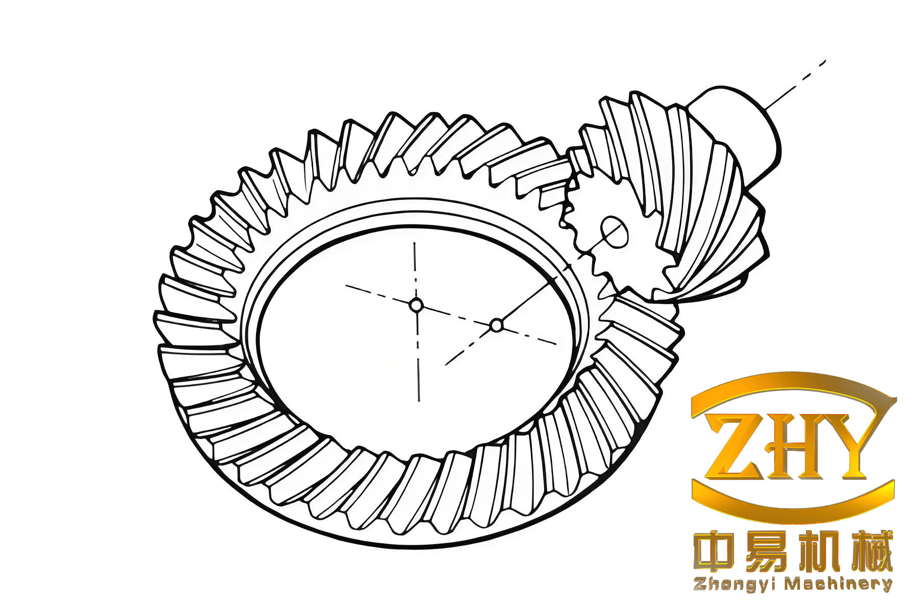
The hypoid bevel gear is widely used in machine tool transmission, aerospace industry, and automotive powertrain systems because it can withstand large stresses, has a high stacking coefficient, produces low transmission noise, causes small power transmission loss, has strong fatigue resistance, and offers high working reliability. The gear pair transmits motion and power between the pinion and the gear through tooth surface meshing. Its working nature determines the stability of the overall working system. The quality of the meshing performance of the hypoid bevel gear directly affects the working quality of the equipment. The transmission stability and transmission noise of a hypoid bevel gear are determined by the morphology of the tooth surface contact area and the amplitude of the transmission error during meshing. During assembly, a hypoid bevel gear pair inevitably exhibits offset distance errors, mounting distance errors of the pinion and gear, shaft angle errors, and other assembly errors. During manufacturing, after cutting, heat treatment, and lapping, tooth surface errors are unavoidable. Installation errors and tooth form errors cause the transmission error of the hypoid bevel gear to increase and the contact area to deviate from the standard region, reducing meshing performance, including transmission quality, service life, and vibration noise.
At the present stage, most research adopts finite element simulation of the hypoid bevel gear pair and improves meshing performance by adjusting installation errors. However, most simulations use a theoretically designed gear pair model, while the rolling experiment validation uses an actually manufactured gear. This again creates the problem of inconsistent evaluation standards. Therefore, to effectively improve the meshing performance of the hypoid bevel gear pair and increase its service life, I start from the reconstruction of real tooth surfaces and study the influence of installation errors on meshing performance. I establish a three-dimensional model for simulation, simulate the relationship between installation errors and the transmission error and contact area of the hypoid bevel gear, and provide optimization suggestions for improving the assembly quality of the main reducer.
Many factors affect the meshing performance of a hypoid bevel gear. Based on previous experience, these factors can be summarized as follows: the location and shape of the tooth surface contact area, the transmission error between gears, and the gear displacement caused by load. The degree of contact area deviation and the variation amplitude of transmission error directly affect the meshing performance of the hypoid bevel gear. Therefore, by adjusting the assembly errors of the gear pair, I can standardize the contact area of the hypoid bevel gear and make the amplitude of the meshing transmission error controllable.
In recent decades, due to the optimization of gear cutting, heat treatment, and lapping processes for hypoid bevel gears, tooth surface machining quality can basically be guaranteed at a good level, and tooth surface machining errors have been controlled to a certain extent. However, in the actual assembly of the main reducer, installation errors occur. It is necessary to manually adjust the gear pair to the ideal installation position by placing adjusting shims in the axial direction of the gear pair, so that the meshing contact area of the hypoid bevel gear is located in the ideal region and the transmission error is not excessive. During assembly, workers rely on subjective judgment, and sometimes multiple disassembly and assembly operations are required. Because the transmission error and meshing contact area of the hypoid bevel gear are highly sensitive to installation errors, finite element simulation of the gear pair to optimize various installation errors and thereby control the transmission error and meshing contact area is efficient and objective. However, at the current stage, most gear pair simulations use theoretically designed gear pair models. Due to the existence of tooth surface errors, the simulation results are not accurate and deviate from the rolling experiment of the actual hypoid bevel gear. Therefore, I start from unifying the evaluation standard of simulation and rolling experiment, and I investigate the influence of assembly errors on the contact area and transmission error. Through reconstruction of real tooth surfaces and finite element simulation, I propose optimization suggestions for the assembly process of the rear axle main reducer, control the transmission error of the hypoid bevel gear, and ensure that the meshing contact area is in a good position, thereby improving the manufacturing performance of the main reducer.
In my research, I mainly study the influence of installation errors on transmission error and meshing contact area. To unify the evaluation standard of simulation and rolling experiment, I reconstruct the real tooth surface of the hypoid bevel gear, obtain a digital real tooth surface model, use this model for simulation, investigate the influence of installation errors on transmission error and meshing contact area, and finally use the influence laws to optimize the assembly work of the main reducer. I optimize the assembly calculation and process flow in the assembly of the main reducer, thereby solving the problem of uneven load distribution on the tooth surface caused by poor contact area during meshing of the hypoid bevel gear, which leads to tooth surface damage and reduced service life. I control the transmission error, reduce the generation of transmission noise, improve the NVH characteristics of the rear axle, and ultimately optimize the performance of the complete vehicle.
To provide a clear summary of the main notation used in my study, I list the key symbols in Table 1.
| Symbol | Meaning |
|---|---|
| $\Delta V$ | Offset distance error of the hypoid bevel gear pair |
| $\Delta H$ | Axial mounting distance error of the pinion |
| $\Delta E$ | Mounting distance error of the gear |
| $\Delta \Sigma$ | Shaft angle error |
| $TE$ | Transmission error |
| $\varphi_1$ | Rotation angle of the pinion |
| $\varphi_2$ | Actual rotation angle of the gear |
| $\varphi_2’$ | Theoretical rotation angle of the gear |
| $Z_1, Z_2$ | Number of teeth of pinion and gear |
I now recall the basic meshing theory of the hypoid bevel gear. A gear tooth surface meshing can be regarded as two kinds of conjugation: local conjugation and complete conjugation. Local conjugation means that the tooth surface $\Sigma_1$ produces a contact spot at each instant, and the contact spots connected together form the contact trace $L_1$ on the tooth surface $\Sigma_1$. The instantaneous relative velocity at each contact point is tangent to the contact trace $L_1$. Complete conjugation means that the tooth surface $\Sigma_1$ produces a contact line at each instant, and the contact area is composed of the combination of contact lines. For a hypoid bevel gear pair, the meshing condition belongs to local conjugation.
For two surfaces $S^{(1)}$ and $S^{(2)}$ in contact, the position vector and unit normal vector must satisfy the following conditions at the contact point $M$:
$$
\begin{cases}
r_2 = m + r_1 \\
n_2 = n_1
\end{cases}
$$
where $r_1$ and $r_2$ are the radius vectors from the origins of the moving coordinate systems to the contact point, $m$ is the vector from $O_1$ to $O_2$, and $n_1$ and $n_2$ are the unit normal vectors. This equation is the meshing equation in the theory of the hypoid bevel gear.
For the hypoid bevel gear, I express the tooth surface as:
$$
r^{(i)} = r^{(i)}(u_i, \theta_i), \quad i=1,2
$$
and the unit normal vector as:
$$
n^{(i)} = \frac{\frac{\partial r^{(i)}}{\partial u_i} \times \frac{\partial r^{(i)}}{\partial \theta_i}}{\left\| \frac{\partial r^{(i)}}{\partial u_i} \times \frac{\partial r^{(i)}}{\partial \theta_i} \right\|}
$$
In the fixed reference coordinate system $S_h$, the ideal contact condition requires that the position vectors and normal vectors of $\Sigma_1$ and $\Sigma_2$ are equal:
$$
\begin{cases}
r_h^{(1)}(u_1, \theta_1, \varphi_1) = r_h^{(2)}(u_2, \theta_2, \varphi_2) \\
n_h^{(1)}(u_1, \theta_1, \varphi_1) = n_h^{(2)}(u_2, \theta_2, \varphi_2)
\end{cases}
$$
Since the meshing of the tooth surfaces is tangent and continuous at each instant, the first derivative with respect to time $t$ must also be equal:
$$
\begin{cases}
\dot{r}_h^{(1)}(u_1, \theta_1, \varphi_1) = \dot{r}_h^{(2)}(u_2, \theta_2, \varphi_2) \\
\dot{n}_h^{(1)}(u_1, \theta_1, \varphi_1) = \dot{n}_h^{(2)}(u_2, \theta_2, \varphi_2)
\end{cases}
$$
According to the meshing theory, the hypoid bevel gear pair must satisfy the following conditions in the same coordinate system: the contact points of the pinion and gear have the same normal vector, the relative velocity is perpendicular to the normal vector, and the radius vectors are equal:
$$
\begin{cases}
\vec{n}_1 = \vec{n}_2 \\
\vec{V} \cdot \vec{n} = 0 \\
\vec{r}_1 = \vec{r}_2
\end{cases}
$$
where $\vec{n}_1$ and $\vec{n}_2$ are the normal vectors at the conjugate contact point of the pinion and gear tooth surfaces, $\vec{V}$ is the relative velocity vector of the gear at the conjugate contact point, and $\vec{r}_1$ and $\vec{r}_2$ are the radius vectors at the conjugate contact point.
Once the midpoint of the contact area is calculated, the entire contact trace can be solved. Let the initial contact point be $M$. After making $u_1$, $u_2$, $\theta_1$, and $\theta_2$ explicit, the meshing trace of the hypoid bevel gear can be easily obtained:
$$
r_p(\theta_1, \varphi_1) = r_g(\theta_2, \varphi_2)
$$
The system contains four unknown parameters and three equations. If the pinion rotation angle $\varphi_1$ is treated as the input parameter, the remaining parameters can be solved by Newton iteration, which helps improve the stability of the calculation. The contact trace on the real tooth surface can be displayed more intuitively in a three-dimensional diagram. To represent the search method for contact points on the tooth surface, it is necessary to project the three-dimensional solid of the tooth surface onto the axial section. For a point $M$ on the tooth surface, its projection onto the design intersection point $C_i$ along the gear axis has distance $E_i$ and distance $D_i$ from the gear axis, satisfying:
$$
\begin{cases}
D_i = |R_i \times P_i| \\
E_i = R_i \cdot P_i
\end{cases}
$$
The pair $(D_i, E_i)$ is derived from the equations formed by $(\theta_2, \varphi_2)$. I can take the reference point $M$ on the contact trace as the initial contact point and calculate other contact points. The specific steps are as follows. First, I take $M$ as the initial contact point, substitute $\varphi_1$ as the first value, and then give a very small step $\Delta \varphi_1$. Using Newton iteration to solve the equations, I obtain the first set of $(u_1, u_2, \theta_1, \theta_2)$. Second, I substitute this set into the tooth surface equations of the pinion and gear to solve the coordinates of the conjugate point. Third, I continuously reduce the step $\Delta \varphi_1$ and repeat the first two processes to obtain all values of the contact line. Fourth, I increase the step $\Delta \varphi_1$ in the other direction. As long as it does not exceed the range of the tooth surface, I obtain all contact points.
Based on the technical parameters of the pinion and gear, I use $M$ as the reference point and adjust the step size to detect the position of the gear surface. Alternatively, I can use MATLAB programming to simulate the contact trace starting from point $M$. For the contact area between the concave surface of the pinion and the convex surface of the gear, the parameters of the contact trace are generally specified as follows: the distance from the contact area to the tooth root is zero, the distance to the tooth tip is zero, the distance to the large end of the pinion is 1.4687, and the distance to the small end is 0. For the contact area between the convex surface of the pinion and the concave surface of the gear, the distance from the contact area to the tooth root is 0.0146, the distance to the tooth tip is zero, the distance to the large end of the pinion is zero, and the distance to the small end is 0.7206. The left side represents the meshing-in stage, the middle represents the full tooth contact stage, and the right side represents the meshing-out stage.
In the actual installation of a hypoid bevel gear pair, deviations from the ideal assembly parameters inevitably occur, and these are called installation errors. The installation errors of a hypoid bevel gear pair are usually divided into four types. The offset distance error $\Delta V$ is the distance between the actual rotation axis of the pinion and the theoretical axis. The pinion axial mounting error $\Delta H$ is the deviation between the actual installation position and the ideal installation position along the rotation center direction of the pinion. The gear axial mounting error $\Delta E$ is the deviation between the actual installation position and the ideal installation position along the rotation center direction of the gear. The shaft angle error $\Delta \Sigma$ is the deviation of the angle between the two gear axes from the standard installation angle.
The transmission error of the hypoid bevel gear is defined as follows. Theoretically, the gear pair transmits motion according to a fixed transmission ratio $i_{21}$:
$$
i_{21} = \frac{\omega_2}{\omega_1} = \frac{Z_1}{Z_2}
$$
where $\omega_2$ is the rotational speed of the gear, $\omega_1$ is the rotational speed of the pinion, and $Z_1$ and $Z_2$ are the numbers of teeth of the pinion and gear, respectively. In the ideal state, the pinion and gear move linearly:
$$
\varphi_2′(\varphi_1) = \frac{Z_1}{Z_2} \varphi_1
$$
where $\varphi_1$ is the rotation angle of the pinion and $\varphi_2’$ is the theoretical rotation angle of the gear. In actual operation, there is a deviation between the theoretical rotation angle $\varphi_2’$ and the actual rotation angle $\varphi_2$ of the gear. In the meshing motion of the hypoid bevel gear pair in the rear axle main reducer, the transmission error is the value obtained by subtracting the theoretical rotation angle from the actual rotation angle of the driven gear after the driving gear rotates by a certain angle. This value varies periodically with the pinion rotation angle, and the curve is the transmission error curve. The transmission error expression is:
$$
TE = \varphi_2(\varphi_1) – \varphi_2′(\varphi_1) = (\varphi_2 – \varphi_2^{(0)}) – \frac{Z_1}{Z_2}(\varphi_1 – \varphi_1^{(0)})
$$
where $\varphi_1^{(0)}$ is the initial rotation angle of the pinion, $\varphi_2^{(0)}$ is the initial rotation angle of the gear, and $Z_1$ and $Z_2$ are the numbers of teeth of the pinion and gear, respectively.
In the actual production of a hypoid bevel gear, after gear cutting, heat treatment, and lapping, tooth profile machining position errors and carburizing structure deformation are unavoidable. There are first-order errors, second-order errors, and higher-order errors. Different types of errors produce different precision errors in the contact area. A first-order error refers to a pressure angle error or a spiral angle error. The pressure angle error reflects the tooth height error in the same direction, while the spiral angle average error reflects the actual error of the tooth length on the tooth surface. Since tooth surface machining errors cannot be removed, and installation errors such as shaft angle error and axial distance error always occur during gear assembly, the meshing contact pattern of the hypoid bevel gear pair must exhibit errors. This causes the gear pair to deviate from the standard contact area that provides the best transmission performance and meshing performance, reducing the meshing transmission performance. The standard contact area and defect types of the contact area include small end contact, large end contact, large and small end contact, tooth root contact, tooth tip contact, tip-root contact, wide contact in the tooth height direction, narrow contact in the tooth height direction, bridge-shaped contact in the tooth height direction, long contact in the tooth length direction, short contact in the tooth length direction, bridge-shaped contact in the tooth length direction, inner diagonal contact, and outer diagonal contact. Because errors exist, the position of the gear meshing contact area shifts, and the shape is not conducive to meshing. Tooth surface errors in the tooth height direction cause the meshing contact area to deviate from the middle position in the tooth height direction. Tooth surface errors in the tooth length direction cause the meshing contact area to deviate from the middle position in the tooth length direction. Usually, tooth surface errors in both the tooth length and tooth height directions exist simultaneously, and their combined effect leads to inner diagonal or outer diagonal conjugation in the paired contact area. In the actual tooth cutting process, the tooth profile also changes the tooth length, tooth height, and curvature, which jointly affect the defects in the contact area shape. Therefore, it is necessary to study and solve the problem of how to correct and control tooth surface errors, avoid contact area defects, and improve the quality of the meshing contact area.
For quality inspection of the hypoid bevel gear, I measure tooth surface roughness using a Taylor Hobson roughness tester. The measurement accuracy of this instrument can reach 0.0001 $\mu$m, and it mainly uses a probe to perform sliding measurement along a specified path on the gear tooth surface. Through the computer equipped with the detection instrument, I can measure various parameter values reflecting tooth surface roughness, such as $R_a$, $R_{sk}$, $R_z$, $R_p$, and $R_v$. For the meshing contact area, I use a 600HTT rolling tester. When inspecting the contact area, I spray red lead pigment on the teeth of the measured gear, adjust the gear to a relatively horizontal position, and keep the rolling gear under the lightest load. At this time, the mark formed by the removal of red lead pigment on the gear surface is called the meshing contact area of the gear. The standard contact pattern of the hypoid bevel gear pair is used as the reference.
The main content of my research includes the following. First, based on the meshing theory of the hypoid bevel gear, I derive the motion relationship equation of tooth surface meshing and solve the equations for the instantaneous contact point and tooth surface contact trace of the gear pair. I analyze the assembly errors and meshing errors that affect the meshing performance of the hypoid bevel gear and clarify the variables that need to be controlled to improve meshing performance. I introduce the detection methods for tooth surface roughness and meshing contact area of the hypoid bevel gear, providing a basis for subsequent measurement of actual tooth surfaces and validation of transmission error and contact area simulations.
Second, I analyze the NURBS curve and surface fitting construction method and derive the generation process of NURBS curve and surface fitting. I import the theoretical tooth surface model into a Gleason 350GMM gear measurement center as the reference surface for measuring the real tooth surface, and I plan the path to measure the real tooth surface parameters. Using the NURBS curve and surface fitting method, I complete the construction of the real tooth surface of the hypoid bevel gear that meets the accuracy requirements and establish a three-dimensional model in CATIA.
Third, I bring the three-dimensional model of the real tooth surface into ABAQUS for simulation analysis. I use Hypermesh to mesh and preprocess the model. By controlling a single variable and adjusting the value of each installation error, I perform simulation analysis and obtain the ranking of the influence of each installation error on transmission error: $\Delta \Sigma = \Delta H > \Delta V > \Delta E$. I use a Gleason 600HTT rolling tester to conduct experiments, verify the rationality of using the real tooth surface reconstruction model for simulation, and summarize the influence of multiple installation errors on transmission error when they act together. Based on the reconstructed tooth surface equation and kinematic meshing contact theory, combined with the influence law of installation errors on transmission error, I use the golden section search method to adjust installation errors to optimize the gear contact area, achieving contact area standardization and controllable transmission error.
Fourth, I combine the simulation results of transmission error and contact pattern to optimize the assembly process of the main reducer. First, through simulation calculation, I obtain a set of installation error combinations that conform to the control interval of transmission error. Then, according to the standardized simulation results of the contact pattern, I obtain the final assembly optimization scheme and optimize the assembly process of the main reducer. Finally, I use a gear rolling machine experiment to verify the reliability of the simulation model.
For the NURBS curve and surface construction, the general rational expression of a $k$-th degree NURBS curve is:
$$
p(u) = \frac{\sum_{i=0}^n \omega_i N_{i,k}(u) d_i}{\sum_{i=0}^n \omega_i N_{i,k}(u)}
$$
where $\omega_i$ are weight factors, $N_{i,k}(u)$ are basis functions, $d_i$ are control vertices, $k$ is the order, and $u$ is the variable. The basis functions are defined recursively as:
$$
\begin{cases}
N_{i,0}(u) = \begin{cases} 1, & u_i \le u \le u_{i+1} \\ 0, & \text{otherwise} \end{cases} \\
N_{i,k}(u) = \frac{u – u_i}{u_{i+k} – u_i} N_{i,k-1}(u) + \frac{u_{i+k+1} – u}{u_{i+k+1} – u_{i+1}} N_{i+1,k-1}(u), \quad k \ge 1
\end{cases}
$$
For the real tooth surface model in my study, the fitting curves are open curves. Therefore, I set the coincidence rate of the two end points to $k+1$, which determines that the end points of the curve coincide with the control points. This also ensures that the first and last edges of the polygon are perpendicular to the first and last points of the fitting curve, simplifying the calculation of the control vertices. For a cubic NURBS curve, the rational expression is:
$$
p(u) = \frac{\sum_{j=i}^{i+3} \omega_j N_{j,3}(u) d_j}{\sum_{j=i}^{i+3} \omega_j N_{j,3}(u)}
$$
After deriving the recursive basis functions and combining them with the above equation, the matrix expression of the cubic NURBS curve is:
$$
p(u) = \frac{U N_i D_i}{U N_i W_i}
$$
where $U = [1, u, u^2, u^3]$, $0 \le u \le 1$, and $N_i$ is a $4 \times 4$ matrix. The NURBS curve is constructed by solving the control vertices through the inverse calculation of the type value points on the curve. For a cubic NURBS surface, the rational expression is:
$$
p(u,v) = \frac{\sum_{i=0}^m \sum_{j=0}^n \omega_{i,j} N_{i,k}(u) N_{j,l}(v) d_{i,j}}{\sum_{i=0}^m \sum_{j=0}^n \omega_{i,j} N_{i,k}(u) N_{j,l}(v)}
$$
To make the real tooth surface construction more concise and improve calculation efficiency, I convert the rational expression of the NURBS surface into a matrix expression. The matrix form of the bicubic NURBS surface is:
$$
p_{i,j}(u,v) = \frac{U N_i D_{i,j}^{\omega} N_j^T V^T}{U N_i \omega_{i,j} N_j^T V^T}
$$
where $U = [1, u, u^2, u^3]$, $V = [1, v, v^2, v^3]$, and $D_{i,j}^{\omega}$ and $\omega_{i,j}$ are matrices related to the control vertices and weight factors.
The inverse calculation of NURBS surface control points is similar to that of NURBS curves, but it requires calculation of control points in both directions. The specific process is as follows. First, I determine the parameter directions. According to the rectangular arrangement of the surface type value points, one boundary direction is the parameter direction of the tooth length, and the other boundary direction is the parameter direction of the tooth width. Second, I calculate the node vectors using the accumulated chord length parameterization method for all curves in the two directions. Third, I inversely calculate the control vertices from the node vectors. For the inverse calculation, I first select type value points in one parameter direction in sequence and use the inverse calculation process of cubic NURBS curve control points to obtain $m$ control points on each cubic NURBS curve. Then I use the control points obtained in the previous step as the type value points in the other parameter direction and again use the control point inverse calculation method to calculate the control points in the other direction. These control points are the control points of the bicubic NURBS surface. Generally, for high-precision surface fitting, the more type value points selected, the better.
For measuring the real tooth surface of the hypoid bevel gear, the planning of the measurement path is crucial. Selecting an appropriate detection path can not only improve the detection data but also ensure the detection effect. First, I import the theoretical tooth surface model of the hypoid bevel gear from the gear design software into the Gleason 350GMM gear measurement center, using the theoretical design tooth surface as the reference surface for measuring the actual tooth surface. Because the tooth surface structure is complex, all points on the gear surface need to be projected onto the rotational projection plane of the transmission gear. Since the research object is a hypoid bevel gear with equal height teeth, the projected image is a standard rectangle. To improve the detection speed of the actual tooth surface and ensure the detection quality of the theoretical tooth surface, I plan the tooth surface grid as follows. The grid nodes for tooth surface detection generally consist of 45 measurement points selected on the tooth surface. Specifically, the tooth length is divided into 9 columns, and the tooth width is divided into 5 columns, so the grid division ratio of tooth surface measurement is 9:5. The grid edges in the tooth width direction must be determined within 5% of the tooth width, and the grid edges in the tooth length direction must be determined within 10% of the tooth length. The distance between grid edges must not exceed 0.7 mm.
At present, the point matrix measurement method is widely used for tooth surface measurement. In this method, when the gear is measured by the probe, the probe measures the grid nodes on the tooth surface one by one along the tooth width and tooth depth directions at predetermined distances. This measurement method can reduce the deviation caused by collision between the probe and the transmission surface. It has high measurement accuracy but slow measurement speed. The measurement process can be summarized as follows. First, I use the meshing node of the theoretical design tooth surface as a reference to guide the probe along the measurement path of the actual tooth surface. Second, I use a computer to calculate the coordinate values of the meshing nodes corresponding to the actual tooth surface, fit the three-dimensional coordinate values to the gear surface, and obtain the actual tooth surface. Third, I compare and analyze the measured actual tooth surface with the previously input theoretical design tooth surface to obtain the deviation of the hypoid bevel gear.
When measuring the concave surface of the pinion tooth surface, using the point matrix measurement method may cause interference between the probe and the gear teeth. When measuring a gear with a large spiral angle, the point matrix detection method may also cause probe slippage and probe breakage. In addition, when measuring the actual tooth surface with the point matrix measurement method, the amount of tooth surface information obtained is relatively small, but as long as the grid division and path planning are done well, the accuracy can be increased. Therefore, the point matrix measurement method is suitable for measuring the actual tooth surface in this work.
To make the horizontal movement of the gear and the measurement of the probe not conflict, the probe can be arranged in a specific way. When measuring the passive gear of a hypoid bevel gear, because the passive gear has many teeth and small tooth surface curvature and a relatively large pitch cone angle, the probe must be arranged vertically to make it easier for the probe to contact the entire tooth surface. When using the point matrix measurement method to detect the tooth surface, it is necessary to plan the detection route, and the probe detects the tooth surface point by point along the specified detection route. Therefore, the specification of the tooth surface detection route is very important. To improve the accuracy of detection data and the detection effect, it is necessary to choose a correct detection route. There are usually two measurement paths. The first measurement path treats the point on the large end or small end of the transmission gear that is closest to the tooth tip as a detection point, and each detection cycle starts from one end and ends at the opposite end. This path can make the rotary table always rotate in the same direction during tooth surface data measurement, effectively reducing the error in surface detection accuracy caused by the rotation angle error of the rotary table. Therefore, this method has higher measurement accuracy but slow measurement speed. The second measurement path uses the midpoint of the actual tooth surface as a reference point and starts measuring from there. Then the probe completes the measurement along an S-shaped measurement path. This method has high measurement efficiency, but the worktable changes frequently, which produces unnecessary errors. Considering all factors, I use the first measurement path planning method to detect the projected tooth surface.
When the actual tooth surface is measured, the measured gear must be placed in the measurement center so that the coordinate system of the gear motion workpiece corresponds to the measurement coordinate system. The design intersection point of the hypoid bevel gear is set at the origin of the gear coordinate system, following the right-hand rule. In addition, the origin of the gear measurement coordinate system can be set on the measuring center worktable, following the left-hand rule. When measuring the rear tooth surface of the passive gear, a special clamping tool is needed to install the rear cone surface of the passive gear on the rotating worktable of the test center. A dial indicator can be used to adjust the fixed point height of the gear so that the main axis of the gear coordinate system coincides with the main axis of the measurement coordinate system. At this time, the difference between the two origins is the fixed point height of the passive gear. After checking the pinion, the pinion must first be positioned through the special center of the gear inspection center. Due to the influence of the special center, the $x_w$ axis of the gear position system naturally coincides with the $z_c$ axis of the measurement position system.
The relationship between the gear coordinate system $S_w(X_w, Y_w, Z_w)$ and the measurement coordinate system $S_c(X_c, Y_c, Z_c)$ is:
$$
\begin{cases}
X_c = -Y_w \\
Y_c = -Z_w \\
Z_c = -X_w \pm d
\end{cases}
$$
where $d$ is the distance between the origins of the gear coordinate system and the measurement coordinate system. Because the reference end face positioning method is used in the detection of the pinion and passive gear of the actual tooth surface, if the actual gear tooth surface measurement position is to be fixed, it is necessary to determine the corresponding position relationship between the measurement coordinate system and the gear coordinate system, and determine the size from the reference plane of the gear calibration position to the rotating worktable and the installation distance of the gear.
When measuring the actual tooth surface of the actual gear, the discrete point coordinate values obtained are actually the coordinates of the probe ball center. Therefore, it is necessary to compensate the radius of the probe ball. The compensation value is input into the gear detection center. In the gear detection center, the compensation value should also be the actual positioning value of the actual tooth surface detection point. The relationship between the coordinate value of the probe ball center, the coordinate value of each node on the surface, and the probe radius is used. The coordinate value of point $M$ on the real tooth surface can be obtained from:
$$
R_i = r_i \pm n \cdot r
$$
where $R_i$ is the actual coordinate value of point $M$ on the actual tooth surface, $r_i$ is the coordinate value of the probe center $M_1$ corresponding to point $M$, $n$ is the unit normal vector at point $M$ on the real tooth surface, and $r$ is the radius of the probe.
After the gear surface detection preparation is completed, I use the Gleason 350GMM three-dimensional coordinate gear surface detection center instrument, select the previously selected measurement method and measurement path, and measure 45 grid points on the measured gear tooth surface. Because the gear tooth surface sizes are different, the distance between adjacent grid nodes is also different, so the selected probe diameter is also different. For the hypoid bevel gear studied in this work, a probe with a diameter of 1 mm is selected to measure the actual tooth surface. During measurement, the probe must be moved along the normal direction of the grid points on the tooth surface. At the same time, to avoid interference between the probe and the adjacent tooth surface and the measured tooth surface, it is necessary to select an appropriate probe insertion direction for each grid measurement point. The selection principle is to make the angle between the end face and tangent plane of the measured point and the probe not greater than $45^\circ$, so as to avoid interference between the probe and the adjacent tooth surface.
The actual tooth surface three-dimensional model fitting and reconstruction process is as follows. First, based on the actual three-dimensional coordinate values of the 45 detection points measured on the convex surface of the pinion and their distribution on the actual tooth surface, I input the coordinate values into a spreadsheet. Then I open CATIA modeling software and construct the type value point grid for reconstructing the real tooth surface. Second, I input the coordinates and use MATLAB programs to calculate the control point values of the NURBS curve. After obtaining all the control points of the tooth surface, I repeat the first step to obtain the control point grid of the pinion convex surface. Third, I adjust the weight factors and control vertices to ensure that the curve and surface are generated realistically, that is, I switch the generative shape design module to the free surface module in CATIA for adjustment. I repeat the above operations to generate the pinion tooth surface based on NURBS fitting. The above steps are the reconstruction process of the hypoid bevel gear based on the three-dimensional coordinates of the real tooth surface. I can reconstruct the real tooth surface of the passive gear through the same steps.
Because the model fits the surface, the actual positions of all control points except the control positions are also calculated by surface fitting. Therefore, it is necessary to verify the fitting accuracy of the reconstructed tooth surface. The main verification steps are as follows. First, I select 45 grid points at the same positions on the tooth surface of the theoretical gear model and reconstruct the tooth surface using the NURBS surface fitting method. Second, I combine every four adjacent points on the reconstructed “real tooth surface” of the theoretical gear and take the center point of each small rectangle. Third, I calculate the maximum normal distance between these points on the theoretical design tooth surface and the corresponding midpoints on the reconstructed tooth surface. The maximum normal distance is the maximum fitting error of the hypoid bevel gear model. Fourth, I take the maximum value of the normal distance for each column (8 columns in total). The reconstruction error of the pinion tooth surface is relatively large, and the reason is that the curvature difference of the pinion tooth surface is relatively large. However, the above deviations do not exceed 0.1 $\mu$m. Therefore, using the discrete coordinate point data of the actual tooth surface measured by the three-coordinate measurement center and then reconstructing the real tooth surface through NURBS surface reconstruction for simulation meets the requirements.
Taking the pinion as an example, I open CATIA, enter the part design module, and establish the rough model of the hypoid bevel gear. Then I input the measured coordinate values and the fitted surface model. By referring to the fitted surface, I remove the excess part of the rough model, thus completing the construction of the pinion tooth surface, including the positive and negative tooth surfaces and the tooth profile. I enter the array module, input the number 10, and use the central axis of the rough model of the hypoid bevel gear as the focus to generate all adjacent teeth with concave and convex surfaces. After completing the detailed processing of all tooth surfaces, I obtain the reconstructed three-dimensional model of the pinion. Repeating the above steps, I obtain the reconstructed model of the gear. In the software, I complete the assembly according to the theoretical installation distance.
For finite element modeling and simulation analysis, I use Hypermesh to mesh the simulation model. To improve calculation efficiency, I set the mesh of the tooth surface part involved in meshing to be finer and of better quality, while the mesh size and quality of the non-meshing part can be relaxed accordingly. This meshing method improves both simulation accuracy and simulation speed. The preprocessing for the finite element analysis of the hypoid bevel gear includes material setting and application of load boundary conditions. These settings directly affect the accuracy of the analysis results. For material setting, both the gear and pinion are made of 20CrMnTi, with elastic modulus $E = 212000$ MPa, Poisson’s ratio $\varepsilon = 0.3$, and density $\rho = 7.8 \times 10^3$ kg/mm$^3$. For load boundary conditions, to facilitate the application of rotational force and torque on the gear, reference points must first be established on the rotating shafts of the pinion and gear, so that the load can be displayed on the tooth surface. At the same time, the degrees of freedom of the pinion and gear except rotation around their own main axes must be strictly controlled. When loading, three analysis steps are required. First, control the other positions of the pinion except the shaft. Second, control the other positions of the gear except the gear shaft and apply torque around the gear shaft. Third, control the remaining degrees of freedom of the driving pinion except the shaft and set the angular velocity of the pinion around the axial direction. The contact type settings are shown in Table 2.
| Parameter | Setting |
|---|---|
| Contact type | Surface-to-surface contact |
| Master surface | Pinion contact tooth surface |
| Slave surface | Gear contact tooth surface |
| Dynamic contact method | Penalty function method |
| Slip formulation | Finite sliding |
| Contact friction coefficient | Kinetic friction coefficient 0.1 |
| Contact control | Explicit dynamics |
To verify the rationality of using the real reconstructed tooth surface for computer simulation, I simulate the transmission error of both a theoretically designed hypoid bevel gear pair and a hypoid bevel gear pair reconstructed from the actual tooth surface. The initial condition is that all installation errors are zero. The simulation results show that the constant part of the transmission error of the theoretical tooth surface gear simulation remains basically at 0, while the constant part of the transmission error of the actual tooth surface gear simulation remains basically at $2.5 \times 10^{-3}$ rad. By shifting the transmission error curves to the x-axis, I obtain the fluctuation amplitude curves. The transmission error fluctuation amplitude of the actual tooth surface gear meshing simulation is much larger than that of the theoretical design tooth surface gear simulation. This proves the existence of tooth surface errors in actual machining.
I study the influence of installation errors on the transmission error of the hypoid bevel gear through simulation analysis. The installation errors can be divided into four categories. If all installation errors are zero, the hypoid bevel gear pair is in the ideal installation position. According to the actual assembly process of the main reducer in the rear drive axle of the vehicle model studied in this work and the tolerance requirements of the main reducer machining, the value ranges of the installation errors are shown in Table 3.
| Installation error | Value range |
|---|---|
| Offset distance error $\Delta V$ / mm | $-0.06$ to $+0.06$ |
| Pinion axial mounting error $\Delta H$ / mm | $-0.06$ to $+0.06$ |
| Gear axial mounting error $\Delta E$ / mm | $-0.06$ to $+0.06$ |
| Shaft angle error $\Delta \Sigma$ / $^\circ$ | $-0.06^\circ$ to $+0.06^\circ$ |
When performing a simulation experiment for one type of installation error, the other types of installation errors must be in the standard installation condition. For example, when simulating the offset distance error $\Delta V$, the other three installation errors should be zero.
For the offset distance error $\Delta V$, I take values of $-0.06$ mm, $-0.04$ mm, $-0.02$ mm, $0.02$ mm, $0.04$ mm, and $0.06$ mm. The simulation results show that when $\Delta V$ increases, the transmission error moves in the positive direction as a whole. When $\Delta V$ takes different values, the fluctuation part of the transmission error is basically similar, especially when it takes negative values. However, when $\Delta V$ takes positive values, the fluctuation amplitude of the transmission error shows a clear difference. This is mainly because the change of the offset distance error $\Delta V$ causes the meshing midpoint to shift in the tooth length direction, and the shift is more sensitive when $\Delta V$ changes in the positive direction.
For the pinion mounting distance error $\Delta H$, I take values of $-0.06$ mm, $-0.04$ mm, $-0.02$ mm, $0.02$ mm, $0.04$ mm, and $0.06$ mm. The simulation results show that the transmission error and the installation error have opposite numerical change directions. When $\Delta H$ increases, the overall amplitude line of the transmission error moves in the negative direction. When $\Delta H$ takes positive values, the amplitude curve of the transmission error is obviously more stable than when it takes negative values. This indicates that a positive pinion mounting distance error can reduce the fluctuation of the transmission error amplitude to a certain extent, but the change in the transmission error amplitude is more obvious, and the phase difference generated at the peak of the transmission error fluctuation part is also large. This is mainly because the change of the positive pinion mounting distance error $\Delta H$ causes the meshing midpoint to deviate in the tooth height direction, and the deviation is more obvious when $\Delta H$ changes in the negative direction.
For the gear mounting distance error $\Delta E$, I take values of $-0.06$ mm, $-0.04$ mm, $-0.02$ mm, $0.02$ mm, $0.04$ mm, and $0.06$ mm. The simulation results show that when $\Delta E$ increases, the overall amplitude line of the transmission error moves in the negative direction. Whether $\Delta E$ increases or decreases, the limit value interval of the simulated transmission error is basically the same, and the maximum or minimum value is almost reached synchronously. The reason is that the gear mounting distance error causes a change in the backlash and hardly causes a shift in the meshing midpoint.
For the shaft angle error $\Delta \Sigma$, I take values of $-0.06^\circ$, $-0.04^\circ$, $-0.02^\circ$, $0.02^\circ$, $0.04^\circ$, and $0.06^\circ$. The simulation results show that the greater the deviation of the shaft angle error $\Delta \Sigma$ from the standard installation position, the greater the deviation of the constant value part of the transmission error. When $\Delta \Sigma$ takes negative values, the fluctuation of the transmission error amplitude curve is small, and when the negative value is small, the transmission error fluctuation is stable and has little effect on transmission. When $\Delta \Sigma$ takes positive values, the fluctuation of the transmission error amplitude curve is large. In summary, as long as $\Delta \Sigma$ changes, the amplitude of the transmission error changes drastically.
By studying the sensitivity of the transmission error, I can clarify the types of installation errors that need to be optimized to control the amplitude of the transmission error. I extract the transmission error amplitudes obtained from the above simulations and plot the peak value versus installation error. The analysis shows that whether $\Delta \Sigma$ and $\Delta H$ are too large or too small, they cause an increase in the transmission error amplitude, and the sensitivity is the highest. Therefore, when performing assembly optimization, $\Delta \Sigma$ and $\Delta H$ should be considered as key factors. The sensitivity of the transmission error to $\Delta E$ is very low, so I no longer consider it in the following research. When the offset distance error $\Delta V$ changes in the positive direction, the transmission error changes greatly, so the positive error of $\Delta V$ should be controlled as much as possible. Finally, I obtain the sensitivity ranking: $\Delta \Sigma = \Delta H > \Delta V > \Delta E$. This ranking is summarized in Table 4.
| Installation error | Sensitivity rank |
|---|---|
| $\Delta \Sigma$ | 1 (highest) |
| $\Delta H$ | 1 (highest) |
| $\Delta V$ | 2 |
| $\Delta E$ | 3 (lowest) |
To further prove the accuracy of the simulation and the rationality of using the real tooth surface reconstruction model for simulation, I conduct rolling experiments on the above simulation content to obtain the actual transmission error under the influence of installation errors. I also bring the theoretical design gear model into the software for simulation to obtain the theoretical tooth surface transmission error value under each installation error condition. Finally, I compare the two simulation results with the actual rolling experiment results to verify the correctness of using the real tooth surface reconstruction model for simulation.
Based on previous experience, a Gleason 600HTT bevel gear rolling tester is often used for rolling experiment verification. This device is simple to operate, has good performance, and provides relatively accurate rolling results. It can simulate and detect the meshing contact area position and size, installation errors, transmission error, and other mechanical transmission conditions and gear meshing performance of spiral bevel gears and other gear pairs in actual meshing transmission. The adjustment mechanism of the device for the installation distance is as follows: the up and down movement of the pinion box controls the offset distance displacement $V$; the displacement of the gear box saddle controls the axial displacement $H$; the displacement of the gear box controls the axial distance $E$ of the gear; and the rotation of the gear box controls the shaft angle $\Sigma$ between the pinion and gear axes. The adjustment accuracy of the experimental device is: displacement adjustment of 0.002 mm and angle adjustment of $2’$. The pinion box speed has two gears: 500 r/min and 1000 r/min.
At the beginning of the experiment, I install the gear at the standard installation distance. Then, by inputting different values on the control panel of the 600HTT rolling tester, the pinion and gear boxes automatically adjust to different positions, thereby changing the values of different installation errors of the gear pair. At the same time, to ensure that the force conditions of the two gears on the rolling machine are the same as those in the finite element simulation, I control the rotation speed of the pinion to be the same as that in the simulation. Then, I adjust the control panel of the rolling tester so that the gear pair completes forward rotation experiments under the following conditions: assembly offset distance $\Delta V = \pm 0.04$ mm, pinion mounting distance error $\Delta H = \pm 0.04$ mm, and shaft angle deviation $\Delta \Sigma = \pm 0.04^\circ$. I record the experimental results of each group. Finally, I compare and analyze the rolling experiment results, the simulation results of the real reconstructed tooth surface model, and the simulation results of the theoretical design tooth surface model. The results for different offset distance errors are shown in Table 5.
| Experiment type | Transmission error amplitude / $\mu$rad at $\Delta V = +0.04$ mm | Transmission error amplitude / $\mu$rad at $\Delta V = -0.04$ mm |
|---|---|---|
| Theoretical design tooth surface | 8.420 | 10.710 |
| Real reconstructed tooth surface | 10.870 | 13.280 |
| Actual manufactured gear | 11.399 | 12.712 |
The results for different pinion mounting distance errors are shown in Table 6.
| Experiment type | Transmission error amplitude / $\mu$rad at $\Delta H = +0.04$ mm | Transmission error amplitude / $\mu$rad at $\Delta H = -0.04$ mm |
|---|---|---|
| Theoretical design tooth surface | 12.390 | 19.780 |
| Real reconstructed tooth surface | 16.510 | 21.330 |
| Actual manufactured gear | 17.252 | 20.902 |
The results for different shaft angle errors are shown in Table 7.
| Experiment type | Transmission error amplitude / $\mu$rad at $\Delta \Sigma = +4”$ | Transmission error amplitude / $\mu$rad at $\Delta \Sigma = -4”$ |
|---|---|---|
| Theoretical design tooth surface | 5.710 | 4.770 |
| Real reconstructed tooth surface | 6.860 | 6.820 |
| Actual manufactured gear | 6.803 | 6.798 |
Through the above comparative experiments, I obtain the following conclusions. First, tooth surface errors truly exist. Compared with the actual rolling experiment and the simulation experiment using the real reconstructed tooth surface as the model, the simulation experiment using the theoretical design tooth surface shows a relatively small transmission error amplitude. This is because after actual machining, tooth surface errors are generated, and the actual gear produces a larger meshing error during meshing transmission. Second, the rationality of using the real tooth surface reconstruction model for simulation is confirmed. By comparing the data in the above tables, I find that the transmission error amplitude of the real tooth surface model simulation is very close to that of the actual gear rolling experiment. Both are much larger than the simulation results of the theoretical design tooth surface model. Therefore, the real tooth surface reconstruction model has high precision, and the simulation results based on it are consistent with actual production and detection conditions, giving high simulation credibility.
According to the actual assembly process of the hypoid bevel gear pair in the rear axle main reducer, if the pinion and gear are assembled normally, the tolerance of the shaft angle $\Delta \Sigma$ between the two gears is $90^\circ \pm 5”$, which is almost negligible. Therefore, its influence on the meshing transmission error of the gear pair is very small. According to the conclusion in the sensitivity analysis, the sensitivity of the gear mounting distance error $\Delta E$ to the meshing transmission error of the hypoid bevel gear pair is low, and its influence is very small. In actual assembly, the passive gear is always assembled with the main reducer housing in a standard manner, the error is very small, and $\Delta E$ is also difficult to adjust. Therefore, I no longer discuss it below. In summary, I study the variation law of the meshing transmission error of the hypoid bevel gear when the offset distance error $\Delta V$ and the pinion mounting distance error $\Delta H$ act together.
To improve the meshing performance of the hypoid bevel gear and enhance the stability of the gear transmission system, and based on the influence of assembly errors on transmission error explored in the previous sections, I study the combined influence of the offset distance error $\Delta V$ and the pinion mounting distance error $\Delta H$ on the transmission error. The positive installation error of the offset distance and the negative installation error of the pinion axial assembly distance should be minimized. Therefore, according to the controlled variable method, I take values for the two installation errors and conduct 9 groups of experiments, as shown in Table 8.
| Experiment number | $\Delta V$ / mm | $\Delta H$ / mm |
|---|---|---|
| 1 | -0.02 | 0.02 |
| 2 | -0.04 | 0.02 |
| 3 | -0.06 | 0.02 |
| 4 | -0.02 | 0.04 |
| 5 | -0.04 | 0.04 |
| 6 | -0.06 | 0.04 |
| 7 | -0.02 | 0.06 |
| 8 | -0.04 | 0.06 |
| 9 | -0.06 | 0.06 |
The simulation results show that when $\Delta H \in (0, +0.04]$ and $\Delta V \in [-0.06, 0]$, the two errors reduce the influence of each other on the constant value of the transmission error to a certain extent, and the constant value of the transmission error is smaller than when each acts alone. When $\Delta H \in (+0.04, +0.06]$ and $\Delta V \in [-0.06, 0]$, the two errors increase the influence of each other on the constant value of the transmission error to a certain extent, and the constant value of the transmission error is larger than when each acts alone.
To show the amplitude fluctuation of the transmission error more intuitively when multiple installation errors act together, I quantify the influence of each installation error combination on the transmission error amplitude. The results are shown in Table 9.
| $\Delta V$ / mm | Transmission error amplitude / $\mu$rad at $\Delta H = 0.02$ mm | Transmission error amplitude / $\mu$rad at $\Delta H = 0.04$ mm | Transmission error amplitude / $\mu$rad at $\Delta H = 0.06$ mm |
|---|---|---|---|
| -0.02 | 11.6 | 10.3 | 2.8 |
| -0.04 | 11.3 | 9.6 | 2.5 |
| -0.06 | 6.7 | 7.4 | 2.9 |
By analyzing the table, I obtain the following conclusions. If the value of the pinion offset distance error $\Delta H$ is relatively small, the more negative the offset distance error $\Delta V$, the smaller the transmission error amplitude. If the value of the pinion offset distance error $\Delta H$ is relatively large, the more negative the offset distance error $\Delta V$, the larger the transmission error amplitude. The peak value of the transmission error shifts to the right as the pinion mounting distance error $\Delta H$ increases.
Through the study of the influence of each installation error on the meshing transmission error of the gear pair, I conclude that when assembling the main reducer gear pair, the installation errors that need to be controlled are the offset distance error $\Delta V$ and the pinion mounting distance error $\Delta H$. Through the rolling experiment, I verify the reliability of using the real tooth surface reconstruction model for simulation. Through the controlled variable method, I conduct 9 groups of simulation experiments and preliminarily summarize the variation law of the meshing transmission error when the offset distance error $\Delta V$ and the pinion mounting distance error $\Delta H$ act together. However, the above research does not consider the influence of installation errors on the meshing contact area of the hypoid bevel gear. It is possible that the transmission error amplitude is small, but the contact area of the gear pair does not meet the standard, so the meshing performance of the hypoid bevel gear still does not reach the ideal state. Therefore, to more accurately propose a scheme for optimizing the meshing performance of the hypoid bevel gear, it is necessary to combine the influence law of installation errors on the contact area and use the parameter optimization of installation errors to control the meshing performance.
I solve for the position of the contact area on the tooth surface. The meshing principle and contact analysis equations of the hypoid bevel gear have been described. If the gear parameters are known and the installation errors of the gear pair are determined, the contact trace and other parameters of the theoretical gear pair can be derived. Substituting the obtained parameters into the tooth surface equation determines the properties of the meshing contact area of the hypoid bevel gear. In principle, the tooth surface of a hypoid bevel gear is a non-extensible surface, so the properties of the contact area cannot be directly quantified on the actual tooth surface. However, the contact area can be projected onto the axial section of the tooth blade for quantitative processing, which allows a relatively accurate and intuitive description of the contact area properties. I use this standard to discuss the results and quantitatively determine the properties of the gear pair contact area on the tooth surface.
Taking the contact area length in the tooth height direction as an example, I can quantify the ratio of the length of the meshing contact area in the tooth height direction to the entire tooth height, that is, the ratio of the distance from the edge of the contact area in the tooth height direction to the tooth root or tooth tip to the entire tooth height, to ensure the standardization of the contact area. The quantification in the tooth length direction is the same. Of course, different standards are required for different types of hypoid bevel gears. The evaluation standard for the standardization of the contact area of the hypoid bevel gear in the rear axle main reducer of the vehicle model studied in this work is shown in Table 10.
| Parameter | Value or range |
|---|---|
| Number of teeth of gear | 43 |
| Number of teeth of pinion | 10 |
| Module | 4.186 |
| Face width / mm | 32.26 |
| Whole tooth height / mm | 8.82 |
| $A$ / mm | 5.38 to 12.90 (1/6 to 1/2.5 of tooth length) |
| $B$ / mm | 12.92 to 21.51 (1/2.5 to 1/1.5 of tooth length) |
| $C$ / mm | 1.26 to 2.21 (1/7 to 1/4 of tooth height) |
| $H$ / mm | 2.94 to 4.41 (1/3 to 1/2 of tooth height) |
The tooth surface boundary is used as a reference, and the position of the contact area on the tooth surface is determined by $A$, $B$, $C$, $H$, and $\Sigma$. When the installation position is determined, the movement lengths $A_x$, $B_x$, $C_x$, and $H_x$ of the contact pattern from the tooth surface middle are also determined. If the installation error changes, $A_x$, $B_x$, $C_x$, and $H_x$ change accordingly. If $A_x$, $B_x$, $C_x$, and $H_x$ are all within the given ratio ranges, the obtained contact pattern meets the general meshing standard. After the basic technical parameters of the hypoid bevel gear are selected, I choose the median values of the $A$, $B$, $C$, and $H$ ratio ranges in the above table to obtain the best predicted values $A_0$, $B_0$, $C_0$, and $H_0$. If $A_x$, $B_x$, $C_x$, and $H_x$ are closer to the best predicted values, then $\Delta V$, $\Delta H$, $\Delta E$, and $\Delta \Sigma$ are more reasonable. I establish the optimization objective function:
$$
F_{\min} = (A_0 + A_x)^2 + (B_0 + B_x)^2 + (C_0 + C_x)^2 + (H_0 + H_x)^2
$$
where $A_x$, $B_x$, $C_x$, and $H_x$ are functions of $\Delta V$, $\Delta H$, $\Delta E$, and $\Delta \Sigma$. In general, the tooth height is much smaller than the tooth length, so $A_x$, $B_x$, and $H_x$ are much larger than $C_x$, and $A_x$, $B_x$, and $H_x$ are not equal. To make the contribution of each independent variable to $F_{\min}$ consistent, I calculate the weight coefficients of the four different independent variables. First, I calculate the weighted average using:
$$
Z = \frac{\sum a_i A_i}{\sum a_i}
$$
where $A_i$ represents the optimal value of a single independent variable and $a_i$ represents the contribution ratio of each independent variable to $F_{\min}$. Since the weighted calculation of each value should be consistent, I set all $a_i$ values to 0.25. After calculating the weighted average, I calculate the weight coefficients using:
$$
K_i = \frac{a_i}{(A_i – Z)^2}
$$
Substituting the above formulas, I obtain the weight coefficients for $A_x$, $B_x$, $C_x$, and $H_x$. Therefore, the objective function becomes:
$$
F_{\min} = k_a (A_0 + A_x)^2 + k_b (B_0 + B_x)^2 + k_c (C_0 + C_x)^2 + k_d (H_0 + H_x)^2
$$
where $k_a$, $k_b$, $k_c$, and $k_d$ are the weight coefficients of $A$, $B$, $C$, and $D$. Since $\Delta V$, $\Delta H$, $\Delta E$, and $\Delta \Sigma$ must be within reasonable adjustment ranges, $V$, $H$, $E$, and $\Sigma$ must satisfy the inequality constraints:
$$
\begin{cases}
V_1 \le V \le V_2 \\
H_1 \le H \le H_2 \\
E_1 \le E \le E_2 \\
\Sigma_1 \le \Sigma \le \Sigma_2
\end{cases}
$$
The purpose of formulating the optimization method is to find the best position of the contact pattern of the gear pair, while also ensuring that the transmission error meets the requirements. In other words, it is a maximum problem in the geometric sense with several independent variables that have specific range restrictions, that is, an inequality-constrained maximum problem. The optimization of the extreme value problem is usually solved by derivatives, but this proposition is not an explicit function, so it is impossible to calculate the maximum by solving derivatives. In addition, there are differences between the hypoid bevel gear itself and the main reducer housing, and uncertainties in working conditions. Therefore, the choice of optimization algorithm is very important. Considering various factors, I use the golden section search method to solve the problem.
According to the assembly characteristics of the main reducer, I choose the golden section search method. The golden section search method is suitable for solving single-variable objective function optimization problems. This algorithm can save many tedious calculations and also meet the calculation accuracy. In general, if values are taken for each installation distance, the tooth surface meshing contact area is determined, and then the objective value of the objective function is determined. The golden section search method first needs to determine the region where the minimum value is located. The main processing steps are as follows. First, I arbitrarily select a pending optimization variable interval $[a, b]$, compare $f(a)$ and $f(b)$, and if $f(a) > f(b)$, then the trend from $a$ to $b$ is downward. If $f(a) \le f(b)$, swap the interval positions of $a$ and $b$, so the trend from $a$ to $b$ is still downward. Second, the downward trend has been determined. Along the downward direction, I select a golden ratio point $c$ and calculate $f(c)$. If $f(c) < f(b)$, the required interval is $[a, b]$. If $f(c) \ge f(b)$, I calculate the minimum point $u$ and $u_{\lim} = b + 1.618034(c – b)$. Third, I compare $f(u)$ and $f(b)$. If $f(u) \ge f(b)$, then $[b, c]$ is the required interval. If $f(u) < f(b)$, then $[a, u]$ is the required interval. If it is between $c$ and $u_{\lim}$ and $f(u) > f(c)$, then the minimum point exists in the interval $[b, u]$. Once the minimum point interval is determined, I can search for the minimum value. If $a$, $b$, and $c$ are known as initial points, and $f(b) < f(a)$ and $f(b) < f(c)$, then $b$ is obviously between $a$ and $c$. Then $a < b < c$. From the interval $(a, c)$, I select a point $d \ne b$ according to the golden ratio. If $b – a > c – b$, then $d$ is in $(a, b)$; otherwise, it is in $(b, c)$. I calculate $f(b)$ and $f(d)$ and verify whether the interval length has reached the minimum using:
$$
\frac{c – a}{b – d} < \varepsilon
$$
If $f(b) < f(d)$, then $d$, $b$, and $c$ are regarded as new $a$, $b$, and $c$ respectively, and the process starts over. Otherwise, $a$, $b$, and $d$ are regarded as new $a$, $b$, and $c$, and the process starts over until the interval length accuracy is satisfied. If $f(d) < f(b)$, then $f(b)$ is taken as the approximate minimum value; otherwise, $f(d)$ is taken as the approximate minimum value.
I apply the golden section search method to optimize a randomly selected set of hypoid bevel gear pairs. That is, given an initial value of a set of installation errors, I simultaneously adjust $\Delta V$ and $\Delta H$ to complete the optimization. The optimization results are shown in Table 11.
| Parameter | Initial value | Adjustment |
|---|---|---|
| $V$ | -0.023 | $\Delta V = 0.011$ |
| $H$ | 0.035 | $\Delta H = -0.05$ |
| $E$ | 0 | 0 |
| $\Sigma$ | 0 | 0 |
I verify the optimization with an example. Based on the parameters of the hypoid bevel gear, I define the optimization goal: quantify the meshing area of the gear pair and specify the standard relative position relationship between the gear meshing contact area and the actual gear tooth surface. Then, based on the gear meshing and assembly principles, I establish the target optimization function that adjusts the meshing contact area of the gear pair by changing the installation errors, thereby achieving standardization of the meshing area. I combine the real reconstructed tooth surface model equation obtained by the NURBS curve and surface fitting method with the target optimization function. Using the real reconstructed gear model as the carrier of simulation optimization, I use the golden section search algorithm to solve the simulation calculation that improves the position of the meshing contact area by changing the installation errors. After determining a set of installation error coefficients, I present the above calculation process through MATLAB programming and import it into CATIA software in IGES file format. In CATIA software, I simulate the optimization process of the contact area.
By analyzing the simulation results using the real reconstructed tooth surface model, I find that the meshing contact area of the gear pair meets the requirements, and the optimized contact area shape is good. To further verify the reliability and accuracy of the mathematical simulation that uses the real reconstructed tooth surface model and adjusts the meshing contact pattern of the gear pair by changing installation errors, it is necessary to carry out actual gear pair rolling verification. I select the actual gear pair that has been reconstructed, use a 600HTT rolling tester to carry out the actual gear rolling experiment, and compare the rolling inspection results with the simulation results after taking photos and recording them. During the experiment, I adjust the parameters of the rolling tester to ensure that the rolling gear is in the lightest load state before conducting the experiment. I observe the pattern of the red lead pigment removed after rolling and record the results. The contact patterns of the actual gear rolling experiment are almost the same as the contact patterns obtained by simulation. This first shows that the real reconstructed tooth surface model has high precision, and using the real reconstructed tooth surface for simulation analysis is reasonable. The simulation results are very close to the actual situation and have high credibility. Furthermore, it shows that it is feasible to adjust the installation errors using the meshing contact pattern of the gear pair as the judgment standard. It also indirectly proves that combining the meshing contact pattern with the meshing transmission error as a quantitative standard for adjusting installation errors can be further studied. The above also simulates the process of optimizing installation errors based on the meshing contact pattern of the gear pair in the assembly optimization example.
I then optimize the assembly of the main reducer. The rear axle main reducer assembly of an automobile is one of the main components of the rear drive axle. The assembly quality of the internal gear pair affects the meshing quality and service life of the hypoid bevel gear to a certain extent, and further affects the transmission stability of the vehicle and even the fuel consumption of the complete vehicle. Based on the research results obtained above on the influence of installation errors on transmission error and on the contact area of the gear pair, I use the real reconstructed tooth surface model for simulation. According to the simulation results, I propose an assembly optimization scheme for the main reducer and verify the reliability of the assembly optimization scheme through a rolling machine experiment.
The differential assembly structure and the main reducer assembly are considered. When assembling the main reducer, the process can be divided into the differential assembly and the main reducer sub-assembly. I analyze the current differential assembly and main reducer sub-assembly processes and find that the current process has problems. By describing the details of the assembly process, I identify the direction that can be optimized, that is, adjusting the installation errors by changing the thickness of several shims.
For the differential assembly, I consider the structure and assembly. In general, the assembly process is as follows. First, a worker installs the side gear, planetary gears, and spherical washers in the differential housing. Based on subjective experience, the technician selects adjusting shims and spherical washers of appropriate thickness, and then manually rotates and adjusts the side gear and planetary gears. If the gear meshing is smooth during rotation, the planetary gears and the wheel axle are riveted together with a cylindrical pin, and the bolts are tightened with a pneumatic wrench to fix the passive gear on the differential housing. By describing the above assembly process, I find that the technician selects the thickness of the adjusting shims and spherical washers entirely based on experience, and cannot ensure the accuracy of the tooth side clearance. However, according to the assembly accuracy requirements, the tooth side clearance is usually specified at 0.1 to 0.2 mm.
For the main reducer sub-assembly, I consider the structure and assembly. The assembly process is briefly described as follows. The outer rings of the upper and lower tapered roller bearings are assembled into the deep interior of the main reducer by interference fit. According to the subjective experience of the technician, shims of a certain thickness for adjusting the pinion mounting distance and preload are selected. The mounting distance adjusting shim and the pinion are installed in the inner ring of the lower tapered roller bearing, and the bearing inner ring and the pinion shaft should be in interference fit. Then, the spacer, preload adjusting shim, and upper tapered roller bearing inner ring are fitted on the pinion shaft. The oil seal is installed in the main reducer housing, and the locking bolt is tightened. The final step is to select and measure the distance adjusting shims at both ends of the main reducer assembly, press the differential assembly and the distance bearing inner rings at both ends of the main reducer assembly into the main reducer housing, and tighten the installation fastening screws on the rolling bearing cover with a constant torque. The preload of the lock nut is generally controlled between 170 and 220 N$\cdot$m.
I determine and calculate the assembly errors. As explained earlier, the assembly accuracy of the main reducer mainly depends on the offset distance error $\Delta V$ and the pinion axial mounting distance error $\Delta H$. In the actual manufacturing process of the main reducer housing, the lower offset distance dimension of the reducer housing is monitored by the SPC statistical process control method. The analysis of the statistical results shows that the lower offset distance of the main reducer housing is usually within a tolerance of 0.02 mm. The relationship between the distance $L_1$ from the bearing surface in the housing to the center of the gear mounting hole, the thickness $e$ of the pinion mounting distance adjusting shim, the standard mounting distance $H$ of the pinion, and the offset distance error $\Delta H$ of the pinion is:
$$
L_1 = \Delta H + H + e
$$
where the standard mounting distance $H$ of the pinion is determined by the assembly requirements, and I take 92 mm in this work.
I optimize the assembly errors of the main reducer. I randomly select 5 groups of hypoid bevel gear pairs and 1 reducer housing. First, according to the requirement of controlling the transmission error interval of the gear, I determine a set of adjustment values for the installation errors. Then, to obtain a better meshing contact area, I realize the numerical calculation of the standard contact area by programming and import the calculation results into CATIA to obtain the simulation results of the contact area. Then I obtain another set of adjustment values for the installation errors. Combining the adjustment values of the two parts, I calculate and select the appropriate shim thickness, so that the contact area of the gear pair in the simulation is good and the transmission error is within the controllable interval. Finally, I test the 5 groups of gears on a Gleason 600HTT rolling machine to prove whether the optimization data is correct.
For assembly optimization based on transmission error, I analyze previous vehicle test data. When the vehicle is in normal driving condition, the main reducer NVH noise is generally lower than 62 dB, and the transmission error is between 8 and 14 $\mu$rad. Therefore, when the amplitude of the transmission error is used as the basis for assembly error optimization, the transmission error of the main reducer gear should be maintained between 8 $\mu$rad and 14 $\mu$rad to meet the noise control standard of the rear axle main reducer. After testing the experimental main reducer housing, the lower offset distance dimension is 24.985 mm. According to the lower offset distance error calculation formula, $\Delta V = -0.015$ mm. Therefore, in the simulation based on the actual tooth surface, the initial value of the offset distance error $\Delta V$ of the gear pair is set to $-0.015$ mm. According to the assembly formula, I select shims of different thicknesses $e$ to change $\Delta H$ and ensure that the transmission error amplitude meets the requirements. I reconstruct five groups of actual real tooth surface models, bring $\Delta V = -0.015$ mm into ABAQUS for simulation, and obtain the pinion mounting distance error $\Delta H$. The results are shown in Table 12.
| Main reducer number | 1# | 2# | 3# | 4# | 5# |
|---|---|---|---|---|---|
| Transmission error amplitude / $\mu$rad | 9.71 | 12.59 | 8.33 | 11.66 | 10.73 |
| Pinion mounting distance error $\Delta H$ / mm | 0.038 | 0.027 | 0.043 | 0.019 | 0.016 |
From the table, I know that using the transmission error amplitude as the limiting standard, I complete the assembly optimization of the main reducer. Although the transmission errors differ greatly, they are still within the amplitude control interval, which also provides initial data for the next step of optimizing the assembly according to the contact area.
For assembly optimization based on the contact area, the position and size of the meshing contact pattern of the gear pair are also important bases for judging the meshing performance of the hypoid bevel gear and the noise performance of the complete vehicle. Although the influence of installation errors on the contact area is very small, the standardization of the contact pattern can make the load distribution on the gear contact surface uniform, increase the stability of gear transmission, reduce damage to the tooth surface, and prolong the service life of the hypoid bevel gear. Combined with the optimization results of assembly based on transmission error, the transmission error amplitude is controllable and the meshing contact area is standardized during gear meshing.
In the previous section, by using the real tooth surface model for simulation and combining with the distance calculation of the main reducer assembly, I obtained various installation error combinations that can make the transmission error amplitude within the controllable interval. Next, I bring the 5 groups of installation error data into the golden section search model. That is, I give the initial values of the offset distance $\Delta V$ and the pinion mounting error $\Delta H$ for the 5 groups of gears respectively. By adjusting the values of $\Delta V$ and $\Delta H$, the meshing contact area in the simulation is located in the optimal region. Through the calculation of the assembly formula, I obtain the thickness of the selected shim $e$. Finally, I carry out rolling experiments on the 5 pairs of gears respectively and record the contact pattern and transmission error. The experimental and adjustment data are shown in Table 13.
| Main reducer number | 1# | 2# | 3# | 4# | 5# |
|---|---|---|---|---|---|
| Initial offset distance $\Delta V$ / mm | -0.015 | -0.015 | -0.015 | -0.015 | -0.015 |
| Initial pinion mounting error $\Delta H$ / mm | 0.038 | 0.027 | 0.043 | 0.019 | 0.016 |
| Adjusted offset distance $\Delta V$ / mm | 0.0011 | 0.0020 | 0.0050 | 0.0045 | 0.023 |
| Adjusted pinion mounting error $\Delta H$ / mm | -0.008 | -0.006 | -0.026 | -0.022 | -0.009 |
| Shim thickness / mm | 1.382 | 1.277 | 1.336 | 1.259 | 1.295 |
| Transmission error amplitude / $\mu$rad | 10.63 | 9.55 | 7.58 | 12.71 | 8.94 |
| Convex contact pattern | Standard | Standard | Standard | Standard | Standard |
| Concave contact pattern | Standard | Standard | Standard | Standard | Standard |
I analyze the process and results in the table. First, using the transmission error amplitude as the limiting standard, I obtain the installation error optimization combination through simulation. Then, I bring the installation error optimization combination as the initial value into the golden section search model to optimize the gear contact area. After simulation, I obtain the optimized installation error combination. Although the second installation error adjustment amount is relatively small, it ensures that the contact pattern of the hypoid bevel gear is within the specified range during meshing. After completing the two installation error optimizations, the shim thickness selected according to the formula has good consistency. Through the rolling experiment, I find that the transmission error amplitude of the gear pair is within the control interval and the contact pattern is in the standard region.
Through the above analysis, I conclude that using the transmission error amplitude and the meshing contact area as the evaluation standards for meshing performance is reliable. The initial installation error value obtained by measuring the housing is directly input into the simulation process. Through the simulation analysis guided by the two standards, I obtain the installation error combination that achieves the best meshing performance and directly output the shim thickness through calculation, avoiding human subjectivity and improving assembly efficiency.
In summary, I have completed the following work and obtained the main research results. Based on kinematics and the meshing equation of conjugate surfaces, I analyzed the motion relationship of gear pair meshing. According to the gear pair meshing principle, I derived the expression equations for the meshing contact point and contact trace of the hypoid bevel gear pair. I analyzed the assembly errors and meshing errors that affect the meshing performance of the hypoid bevel gear and provided quantitative explanations. I introduced the detection methods for tooth surface roughness and meshing contact area of the hypoid bevel gear.
I analyzed the NURBS curve and surface fitting construction method and derived the generation process of NURBS curve and surface fitting. I imported the theoretical tooth surface model into a Gleason 350GMM gear measurement center as the reference surface for measuring the real tooth surface, and I planned the path to measure the real tooth surface parameters. Using the NURBS curve and surface fitting method, I completed the construction of the real tooth surface of the hypoid bevel gear that meets the accuracy requirements and established a three-dimensional model in CATIA.
I brought the three-dimensional model of the real tooth surface into ABAQUS for simulation analysis. I used Hypermesh for model meshing and preprocessing. By adjusting the values of installation errors and analyzing the simulation results, I obtained the ranking of the influence of installation errors on transmission error: $\Delta \Sigma = \Delta H > \Delta V > \Delta E$. I used a Gleason 600HTT rolling tester to conduct experiments and verified the rationality of using the real reconstructed tooth surface model for simulation. I summarized the influence of multiple installation errors on transmission error when they act together. Through the reconstructed tooth surface equation and kinematic meshing contact theory, combined with the influence law of installation errors on transmission error, I used the golden section search method to adjust installation errors to optimize the meshing contact area, achieving contact area standardization and controllable transmission error amplitude.
I used transmission error and contact pattern as evaluation standards for simulation calculation to optimize the assembly process of the main reducer. First, through simulation calculation, I obtained a set of installation error optimization combinations that conform to the transmission error amplitude control interval. Then, according to the contact range of the pattern, I obtained the final installation error optimization combination scheme. I optimized the assembly of the main reducer and finally used a rolling tester experiment for verification analysis. The results show that using transmission error and contact area as the basis for assembly optimization of the main reducer is beneficial for improving the assembly efficiency of the main reducer. The simulation results obtained using the real reconstructed tooth surface model are almost the same as the results of the actual rolling experiment. Therefore, the assembly optimization scheme proposed based on the simulation results is credible, reasonable, and accurate.
For future work, due to the limitations of experimental conditions, I did not conduct NVH experiments on the complete vehicle, so I did not further investigate the influence of hypoid bevel gear meshing performance on vehicle noise. I also did not analyze contact stress. In future work, the relationship between meshing stress and meshing contact area can be explored to provide a theoretical and practical basis for further improving the meshing performance of the hypoid bevel gear.