
I studied a cycloid-tooth hypoid bevel gear pair used in rear-drive axle main reducers because this type of hypoid bevel gear combines high load capacity, smooth meshing, and low noise. In my work, I treated the hypoid bevel gear as a complete engineering chain: carburizing and quenching, heat-treatment distortion, reverse reconstruction of the distorted tooth surface, dynamic contact simulation under several vehicle operating conditions, and experimental validation. The central problem I addressed was that a hypoid bevel gear with a complex tooth surface does not deform uniformly during heat treatment. The cooling medium flow around the tooth surface changes the local heat transfer coefficient, and this change directly affects carbon diffusion, phase transformation, hardness, residual stress, and geometric distortion. Therefore, I did not use a single static quench boundary condition. Instead, I divided the hypoid bevel gear into inner bore, tooth surface, outer ring, and bottom face regions and applied region-dependent dynamic heat transfer coefficients during quenching.
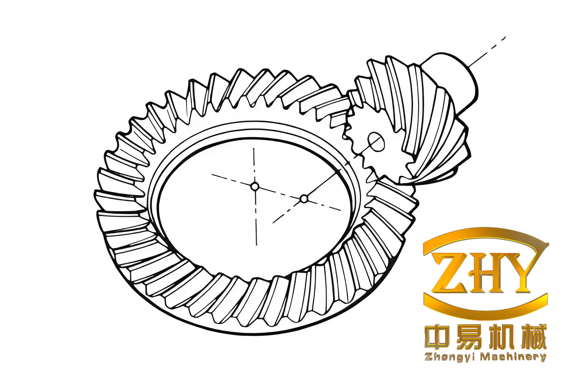
I selected 20CrMoH as the hypoid bevel gear material because it is widely used for gears that require a hard surface and a tough core. The nominal chemical composition I used is listed in the following table. I then calculated the phase transformation temperatures and thermophysical properties with a material simulation tool. This step was necessary because the available property data for 20CrMoH are incomplete for a full coupled heat-treatment simulation.
| Element | C | Mn | Ni | P | S | Mo | Cr | Si | Fe |
|---|---|---|---|---|---|---|---|---|---|
| Mass fraction / % | 0.20 | 0.82 | 0.10 | 0.01 | 0.01 | 0.20 | 1.07 | 0.25 | Balance |
The basic geometry of the hypoid bevel gear pair is summarized below. I used a ring gear with 47 teeth and a pinion with 11 teeth. The shaft angle was 90 degrees, and the offset was 30 mm. The hypoid bevel gear pair therefore had a non-intersecting axis arrangement, which is typical for automotive rear axles.
| Parameter | Ring gear | Pinion | Symbol / unit |
|---|---|---|---|
| Number of teeth | 47 | 11 | z |
| Reference normal module | 3.15216 | 3.15216 | m_n / mm |
| Reference spiral angle | 30.667 RH | 50 LH | beta_m / deg |
| Shaft angle | 90 | 90 | Sigma / deg |
| Face width | 32 | 36.69 | b / mm |
| Offset | 30 | 30 | E / mm |
| Pitch cone angle | 68.633 | 20.25 | delta / deg |
| Reference pitch radius | 86.12 | 26.97 | R_m / mm |
| Addendum | 1.07 | 5.23 | h_a / mm |
| Dedendum | 6.23 | 2.07 | h_f / mm |
For the heat-treatment simulation, I used a process route consisting of preheating, pre-carburizing, strong carburizing, diffusion, holding, oil quenching, and tempering. The holding stage before quenching was important because it reduced the thermal gradient through the hypoid bevel gear while maintaining the surface carbon potential. The quenching oil temperature was kept between 80 and 100 degrees Celsius, and the tempering stage was performed between 170 and 190 degrees Celsius. The full process schedule I adopted is given below.
| Stage | Temperature / deg C | Carbon potential / % | Time / s | Purpose |
|---|---|---|---|---|
| Preheat | 860-880 | None | 3600 | Thermal stabilization |
| Pre-carburizing | 900-920 | 1.00 | 10800 | Initial carbon layer |
| Strong carburizing | 920-930 | 1.15 | 9000 | Surface carbon enrichment |
| Diffusion | 900-880 | 0.90 | 7200 | Homogenize carbon profile |
| Holding | 870-850 | 0.90 | 600 | Prepare for quenching |
| Oil quenching | 80-100 | None | 1200 | Martensitic transformation |
| Tempering | 170-190 | None | 3600 | Reduce residual stress |
I described the coupled heat-treatment problem through temperature, carbon diffusion, phase transformation, stress, and strain fields. The austenite formation during heating can be represented in a simplified form as
$$ \beta_A = 1 – \exp\left[-\left(\frac{T-T_s}{T_e-T_s}\right)^4\right] $$
where \(T\) is the local temperature, \(T_s\) is the lower critical temperature, and \(T_e\) is the upper critical temperature. The martensite volume fraction during quenching was calculated from the temperature-dependent relation
$$ \beta_M = \frac{1-\beta_F-\beta_P-\beta_B}{1-\exp[-0.011(M_s-T)]} $$
where \(\beta_F\), \(\beta_P\), and \(\beta_B\) are the ferrite, pearlite, and bainite volume fractions, and \(M_s\) is the martensite start temperature. For diffusion-controlled transformations, I used the Johnson-Mehl-Avrami-Kolmogorov equation in the incremental form
$$ \beta = 1 – \exp(-k t^n) $$
and the carbon diffusion in austenite followed Fick’s law. I wrote the carbon flux in the simplified one-dimensional form as
$$ J = -D \frac{\partial c}{\partial x} $$
where \(J\) is the carbon flux, \(D\) is the carbon diffusion coefficient, \(c\) is the carbon concentration, and \(x\) is the distance. The heat conduction equation including latent heat was written as
$$ \rho C_p \dot{T} = \nabla \cdot (k_T \nabla T) + \Delta H_F \dot{\beta}_F + \Delta H_P \dot{\beta}_P + \Delta H_B \dot{\beta}_B + \Delta H_M \dot{\beta}_M $$
where \(\rho\) is density, \(C_p\) is specific heat, \(k_T\) is thermal conductivity, and \(\Delta H\) terms are transformation latent heats. The surface heat exchange is governed by
$$ q = h (T_e – T_s) $$
where \(q\) is heat flux, \(h\) is the heat transfer coefficient, \(T_e\) is the external medium temperature, and \(T_s\) is the surface temperature. For the mechanical response, I used the incremental strain decomposition
$$ d\varepsilon = d\varepsilon_e + d\varepsilon_p + d\varepsilon_{th} + d\varepsilon_{tr} $$
where the total strain increment contains elastic, plastic, thermal, and transformation components. The flow stress depended on temperature, carbon content, hardness, and equivalent plastic strain:
$$ Y = Y(T,C,H,\bar{\varepsilon}_p) $$
For hardness prediction, I combined the phase fractions with their individual hardness values:
$$ H = \omega_A H_A + \omega_F H_F + \omega_P H_P + \omega_B H_B + \omega_M H_M $$
The martensite hardness was treated as a function of carbon content, while the other phase hardness values were taken from the material database. This allowed me to predict the hardness distribution after quenching and tempering. The tempering hardness was estimated with a tempered-parameter approach,
$$ H = H_1 + \left(\frac{dH}{dT}\right)\left[\frac{T(273+\log t)}{C}\right] $$
where \(H_1\) is the as-quenched hardness, \(t\) is tempering time, and \(C\) is the Hollomon-Jaffe constant. I used these equations to build a coupled heat-treatment model for the hypoid bevel gear. Because the tooth geometry is complex, a single uniform quench boundary condition would have been unrealistic. I therefore divided the hypoid bevel gear into four surface zones: inner bore, tooth surface, outer ring, and bottom face. The quench oil flow velocities at these zones were different, so the heat transfer coefficients were different. The measured average velocities I used are shown below.
| Medium velocity / (m/s) | Inner bore / (m/s) | Tooth surface / (m/s) | Outer ring / (m/s) | Bottom face / (m/s) |
|---|---|---|---|---|
| 0.4 | 0.1245 | 0.0936 | 0.0607 | 0.0397 |
| 0.8 | 0.2481 | 0.1896 | 0.1694 | 0.1005 |
| 1.2 | 0.4537 | 0.3428 | 0.3189 | 0.1564 |
| 1.6 | 0.5662 | 0.4721 | 0.4813 | 0.1785 |
The heat transfer coefficient curves were selected according to the local flow velocity. In my quench model, the heat transfer coefficient \(h\) varied with surface temperature and velocity. A higher velocity generally increased \(h\) because the vapor film broke down more easily, but an excessively high velocity could create bubbles that reduced the effective cooling rate and produced soft spots. I therefore limited the quench oil velocity below 0.600 m/s for the hypoid bevel gear. The dynamic boundary condition was applied region by region, which made the simulation closer to industrial quenching than a uniform coefficient model.
I used the material simulation results for 20CrMoH to define the elastic and thermal properties. The Poisson ratio and Young’s modulus varied with temperature, as summarized below.
| Temperature / deg C | Poisson ratio | Young’s modulus / GPa |
|---|---|---|
| 0 | 0.290 | 210 |
| 300 | 0.301 | 193 |
| 600 | 0.319 | 152 |
| 900 | 0.345 | 117 |
The transformation temperatures I used for the hypoid bevel gear are listed below. Pearlite began to transform to austenite at 739.4 degrees Celsius, ferrite began to transform at 816.0 degrees Celsius, bainite transformation started at 593.1 degrees Celsius, and martensite transformation started at 402.6 degrees Celsius. These values were essential for predicting the final phase distribution.
| Transformation | Temperature / deg C |
|---|---|
| Pearlite to austenite start | 739.4 |
| Ferrite to austenite start | 816.0 |
| Bainite start | 593.1 |
| Martensite start | 402.6 |
The carbon concentration after each carburizing stage is one of the most important results of the heat-treatment simulation. I extracted the carbon content at the tooth surface, tooth tip, tooth root, bottom face, and core. The tooth tip always had the highest carbon content because of the sharp-corner effect. The tooth root had a lower carbon content because it was located in a more shielded region. The core had the lowest carbon content because carbon diffusion from the surface to the core is slow during the relatively short carburizing cycle. The carbon concentrations after the main stages are given below.
| Stage | Tooth surface / % | Tooth tip / % | Tooth root / % | Bottom face / % | Core / % |
|---|---|---|---|---|---|
| Pre-carburizing end | 0.703 | 0.761 | 0.595 | 0.702 | 0.225 |
| Strong carburizing end | 0.853 | 0.955 | 0.781 | 0.824 | 0.227 |
| Diffusion end | 0.751 | 0.863 | 0.660 | 0.751 | 0.2302 |
| Holding end | 0.756 | 0.851 | 0.656 | 0.745 | 0.2306 |
I found that the tooth surface and bottom face had similar carbon contents because their local geometry did not change as sharply as the tooth tip. The tooth tip reached the highest carbon level during every stage, and the strong carburizing stage produced the maximum surface carbon content. The diffusion stage reduced the surface carbon content and smoothed the carbon profile, which is necessary for avoiding excessive retained austenite and carbide networks. The holding stage kept the carbon profile nearly stable before quenching.
The temperature evolution during quenching controlled the phase transformation. I extracted the cooling behavior of the tooth tip, tooth surface, tooth root, bottom face, and core of the hypoid bevel gear. The tooth tip cooled fastest because it contacted the quench oil directly and had a small thermal mass. The tooth surface was next, followed by the tooth root and bottom face. The core cooled slowest because heat had to be transferred from the interior to the surface. The approximate martensite start times and cooling characteristics are summarized below.
| Region | Relative cooling rate | Approximate martensite start time / s | Typical final temperature after long quench / deg C |
|---|---|---|---|
| Tooth tip | Highest | 1.3 | Lowest among surface regions |
| Tooth surface | High | 2.2 | Close to tip |
| Tooth root | Moderate | 8.0 | Higher than surface |
| Bottom face | Moderate to low | 10.1 | Higher than root |
| Core | Lowest | 15.8 | Highest |
After about 100 seconds of quenching, the temperature differences among the tooth tip, tooth surface, and tooth root were around 11 degrees Celsius, and the difference between the bottom face and core was around 6 degrees Celsius. The maximum temperature difference within the hypoid bevel gear was approximately 50 degrees Celsius. This temperature gradient is the source of thermal stress and distortion. The phase transformation also released latent heat, which temporarily slowed the local cooling rate and influenced the final martensite fraction.
The microstructure and hardness distributions followed the cooling-rate distribution. The tooth tip had the highest martensite fraction and the highest hardness. The tooth surface had slightly lower martensite and hardness. The tooth root, bottom face, and core had progressively lower martensite fractions and lower hardness. The predicted martensite volume fractions and hardness values are listed below.
| Region | Hardness / HRC | Martensite volume fraction |
|---|---|---|
| Tooth tip | 60.42 | 0.982 |
| Tooth surface | 59.33 | 0.974 |
| Tooth root | 51.81 | 0.830 |
| Bottom face | 52.46 | 0.795 |
| Core | 37.8 | 0.636 |
This distribution is exactly the hard-surface and tough-core condition required for a hypoid bevel gear. A high-carbon plate-like martensite with a small amount of retained austenite is desirable near the surface because it provides wear resistance and fatigue resistance. A low-carbon lath martensite with some bainite or retained austenite is desirable in the core because it provides toughness and supports the surface layer. The predicted surface and core hardness values also satisfied the industrial heat-treatment requirements, as shown below.
| Item | Simulated value | Process requirement |
|---|---|---|
| Tooth surface hardness / HRC | 59.33 | 58-64 |
| Core hardness / HRC | 37.8 | 32-45 |
| Bore ellipticity / mm | 0.024 | < 0.07 |
| Inner and outer bottom flatness / mm | 0.028 | < 0.07 |
The residual stress during quenching changed sign as the hypoid bevel gear cooled. In the early stage, the surface cooled faster than the core and contracted, so the surface was in tension while the core was in compression. In the intermediate stage, martensite formation expanded the surface, and the core continued to cool and contract. As a result, the surface stress changed from tension to compression, while the core changed from compression to tension. After the quench, the tooth surface had compressive residual stress and the core had tensile residual stress. This residual stress state is beneficial for contact fatigue because compressive stress near the surface suppresses crack initiation.
The distortion result was not uniform. I found larger thermal distortion near the root of the concave flank at the heel, the middle of the tooth tip, and the root of the convex flank at the toe. These regions are near geometric transitions and therefore experience non-uniform contraction. The middle of the tooth tip formed a slightly raised crown region under the combined action of thermal stress and transformation stress. I marked the crown region using a strain threshold of about 5 micrometers. The measured crown length on the hypoid bevel gear was approximately 23.136 mm. If this crown region becomes too large, the hypoid bevel gear may experience edge contact, which produces impact loads and noise. Therefore, the heat-treatment distortion must be considered in the subsequent meshing analysis.
After the heat-treatment simulation, I reconstructed the distorted hypoid bevel gear tooth surface through reverse engineering. I exported the post-heat-treatment point cloud from the heat-treatment simulation. The initial point cloud contained 9735 points. To reduce computation time without losing tooth-surface accuracy, I simplified the point cloud by setting a distance tolerance. The simplified point cloud contained 6405 points, which was about 34 percent fewer than the original point cloud. I then smoothed the point cloud, removed outliers, and divided the point cloud into concave flank, convex flank, and gear body regions.
| Point-cloud operation | Method | Effect |
|---|---|---|
| Import and inspection | STL point cloud import | 9735 points; maximum span 33.5949 mm |
| Simplification | Distance tolerance of 1 | 6405 points retained |
| Smoothing | Gaussian filter for flanks; median filter for body | Reduced noise and burrs |
| Segmentation | Surface and boundary splitting | Separated concave and convex flanks |
| Curve interpolation | Section curves and NURBS fitting | Prepared closed flank surfaces |
For the concave flank, the lateral deviation, negative deviation, geometric deviation, and positive normal deviation were analyzed. The maximum values are shown below. The maximum geometric deviation was 0.0519 mm, and the maximum negative deviation was -0.0519 mm. These values were much smaller than the allowable threshold.
| Deviation type | Maximum | Mean | Standard deviation |
|---|---|---|---|
| Lateral deviation | 0.0023 | 0.0000 | 0.0001 |
| Negative direction deviation | -0.0519 | -0.0293 | 0.0122 |
| Geometric deviation | 0.0519 | 0.0292 | 0.0123 |
| Positive normal deviation | 0.0017 | 0.0017 | 0.0275 |
For the convex flank, the deviations were also small. The maximum geometric deviation was 0.0447 mm, and the maximum positive normal deviation was 0.0200 mm. Since the hypoid bevel gear diameter was 203.82 mm, a deviation limit of 0.5 percent of the diameter equals 1.0191 mm. All reconstructed flank deviations were below this limit, so I classified the reverse reconstruction as a high-accuracy model suitable for subsequent dynamic contact analysis.
| Deviation type | Maximum | Mean | Standard deviation |
|---|---|---|---|
| Lateral deviation | 0.0000 | 0.0000 | 0.0000 |
| Negative direction deviation | -0.0447 | -0.0146 | 0.0100 |
| Geometric deviation | 0.0447 | 0.0125 | 0.0091 |
| Positive normal deviation | 0.0200 | 0.0091 | 0.0068 |
I rebuilt the full hypoid bevel gear model in a three-dimensional CAD environment. I imported the reconstructed concave and convex surfaces, created the addendum and dedendum cones, trimmed and merged the surfaces, formed one tooth slot, and then used rotation and Boolean operations to generate the complete ring gear and pinion. I checked the assembly for interference. No hard interference was found. I then exported the assembly to a multibody dynamics environment and defined contact between the hypoid bevel gear flanks.
For the transmission error analysis, I used an impact-function contact model. The force exponent was 1.5, the stiffness coefficient was \(3.16 \times 10^9\), the damping coefficient was \(5 \times 10^4\), the static friction coefficient was 0.08, the dynamic friction coefficient was 0.05, the static slip velocity was 0.0001, the dynamic slip velocity was 0.01, and the penetration depth was 0.0001. These parameters are summarized below.
| Contact parameter | Value |
|---|---|
| Force exponent | 1.5 |
| Damping coefficient | \(5 \times 10^4\) |
| Stiffness coefficient | \(3.16 \times 10^9\) |
| Static slip velocity | 0.0001 |
| Static friction coefficient | 0.08 |
| Dynamic slip velocity | 0.01 |
| Dynamic friction coefficient | 0.05 |
| Penetration depth | 0.0001 |
I studied four operating conditions: forward driving, reverse driving, neutral forward rolling, and neutral reverse rolling. In forward and reverse driving, the pinion was the driving member and the ring gear was the driven member. In neutral forward and neutral reverse rolling, the ring gear was the driving member and the pinion was the driven member. The theoretical gear ratio was 4.2727. For forward and reverse driving, the pinion speed was 900 degrees per second and the ring gear torque was 1025 N m. For neutral rolling, the ring gear speed was 211 degrees per second and the pinion torque was 240 N m. The transmission error was evaluated from the difference between the simulated average output speed and the theoretical output speed.
| Condition | Driving member | Driven member | Input speed / (deg/s) | Torque / (N m) | Theoretical output speed / (deg/s) |
|---|---|---|---|---|---|
| Forward driving | Pinion concave | Ring gear convex | 900 | 1025 | 210.638 |
| Reverse driving | Pinion convex | Ring gear concave | 900 | 1025 | 210.638 |
| Neutral forward | Ring gear concave | Pinion convex | 211 | 240 | 901.545 |
| Neutral reverse | Ring gear convex | Pinion concave | 211 | 240 | 901.545 |
The transmission error results are shown below. In forward driving, the maximum output speed was 247.9174 degrees per second, the average output speed was 210.6575 degrees per second, and the minimum output speed was 183.00349 degrees per second. The average speed error was 0.0195 degrees per second, which was a relative error of 0.01 percent. In reverse driving, the maximum output speed was 236.7192 degrees per second, the average output speed was 210.5223 degrees per second, and the minimum output speed was 188.3092 degrees per second. The average speed error was -0.1157 degrees per second, which was a relative error of 0.05 percent.
| Condition | Maximum speed / (deg/s) | Average speed / (deg/s) | Minimum speed / (deg/s) | Average error / (deg/s) | Relative error / % |
|---|---|---|---|---|---|
| Forward driving | 247.9174 | 210.6575 | 183.00349 | 0.0195 | 0.01 |
| Reverse driving | 236.7192 | 210.5223 | 188.3092 | -0.1157 | 0.05 |
| Neutral forward | 1187.7295 | 900.3571 | 661.9666 | -1.1879 | 0.13 |
| Neutral reverse | 1075.5680 | 901.1479 | 745.8160 | -0.3971 | 0.04 |
In neutral forward rolling, the maximum output speed was 1187.7295 degrees per second, the average output speed was 900.3571 degrees per second, and the minimum output speed was 661.9666 degrees per second. The average speed error was -1.1879 degrees per second, which was a relative error of 0.13 percent. In neutral reverse rolling, the maximum output speed was 1075.5680 degrees per second, the average output speed was 901.1479 degrees per second, and the minimum output speed was 745.8160 degrees per second. The average speed error was -0.3971 degrees per second, which was a relative error of 0.04 percent. All four relative errors were below 0.13 percent. The hypoid bevel gear pair was more stable when the pinion drove the ring gear, which agrees with the normal automotive driving arrangement. The neutral rolling cases had larger speed fluctuations, which indicates that driving the pinion through the ring gear is less stable.
For the contact stress analysis, I used an explicit dynamic finite element approach. I first imported the reconstructed hypoid bevel gear model into a professional meshing environment. I cut one tooth sector from the ring gear and one tooth sector from the pinion, refined the tooth-surface mesh, and coarsened the body mesh. I then rotated and copied the meshed sectors to form the full hypoid bevel gear pair. The material properties assigned to the hypoid bevel gear were an elastic modulus of \(2.10 \times 10^{11}\) Pa, a density of \(7.84 \times 10^3\) kg/m\(^3\), and a Poisson ratio of 0.278. The contact definition is summarized below.
| Contact setting | Selection |
|---|---|
| Master surface | Pinion tooth surface |
| Slave surface | Ring gear tooth surface |
| Contact type | Surface-to-surface contact |
| Solver control | Explicit dynamic |
| Friction model | Dynamic friction |
| Contact algorithm | Penalty method |
| Sliding formulation | Finite sliding |
| Friction coefficient | 0.3 |
The normal contact behavior was hard contact, and the tangential behavior was Coulomb friction. The equivalent shear stress was evaluated from two tangential components as
$$ \tau_{eq} = \sqrt{\tau_1^2 + \tau_2^2} $$
The critical shear stress for sliding was
$$ \tau_{crit} = \min(\mu p, \tau_{max}) $$
where \(\mu\) is the friction coefficient, \(p\) is contact pressure, and \(\tau_{max}\) is the material shear yield strength. I applied the load gradually with an amplitude curve so that the contact force did not introduce an artificial impact at the beginning of the simulation. The load ramped from zero to the target value within the first millisecond and then remained constant.
| Condition | Driving surface | Driven surface | Speed / (rad/s) | Torque / (N mm) |
|---|---|---|---|---|
| Forward driving | Pinion concave | Ring gear convex | 104.667 | 1025 |
| Reverse driving | Pinion convex | Ring gear concave | 104.667 | 1025 |
| Neutral forward | Ring gear concave | Pinion convex | 24.492 | 240 |
| Neutral reverse | Ring gear convex | Pinion concave | 24.492 | 240 |
In forward driving, I observed four pairs of teeth in contact at the same time. The contact stress locations formed a staggered pattern along the tooth surface, which explains the high contact ratio and high load capacity of the hypoid bevel gear. The contact force fluctuated between approximately 10 and 20 kN at the beginning and then stabilized around 18 kN. The contact area fluctuated mainly between 40 and 80 mm\(^2\). The periodicity became clearer as the simulation progressed, and the hypoid bevel gear pair behaved in a relatively stable manner.
| Condition | Number of contacting tooth pairs | Contact force range / kN | Contact area range / mm\(^2\) | Stability observation |
|---|---|---|---|---|
| Forward driving | 4 | 10-20, stable near 18 | 40-80 | Small fluctuation, clear periodicity |
| Reverse driving | 4 | 0-40 | 0-95, later 10-85 | Noticeable impact pulses |
| Neutral forward | 3 | 40-140, stable near 90 | 60-160 | Large force and wide fluctuation |
| Neutral reverse | 3 | 20-70 | 40-120 | Moderate but unstable |
In reverse driving, the hypoid bevel gear also had four contacting tooth pairs. The contact force showed intermittent pulses, with values ranging from about 0 to 40 kN. The contact area first ranged from about 0 to 95 mm\(^2\), and later became more concentrated between 10 and 85 mm\(^2\). The impact level was higher than in forward driving, but lower than in neutral forward rolling. In neutral forward rolling, only three tooth pairs carried the load. The contact force was much larger and ranged from about 40 to 140 kN, then stabilized around 90 kN. The contact area ranged from about 60 to 160 mm\(^2\). This condition produced the strongest impact and the largest risk of tooth-surface damage. In neutral reverse rolling, three tooth pairs were also in contact. The contact force ranged from about 20 to 70 kN, and the contact area ranged from about 40 to 120 mm\(^2\). This condition was less severe than neutral forward rolling but still less stable than forward driving.
I concluded from the dynamic contact results that forward driving is the most favorable condition for the hypoid bevel gear. The contact force is small and stable, and the contact area fluctuates within a narrow range with clear periodicity. Reverse driving is acceptable but produces more impact. Neutral forward and neutral reverse rolling are unfavorable because the contact force and contact area fluctuate widely, indicating severe impact and a higher probability of hypoid bevel gear damage.
I validated the numerical model experimentally. I performed carburizing, quenching, and tempering on a hypoid bevel gear made of 20CrMoH in a continuous heat-treatment furnace. After heat treatment, I measured the surface hardness and core hardness with a Rockwell hardness tester. I also examined the microstructure with a scanning electron microscope. The measured surface hardness was about 59.2 HRC, while the predicted surface hardness was about 59.33 HRC. The measured core hardness was about 37.8 HRC, while the predicted core hardness was about 36.9 to 37.8 HRC. The differences were small, which supported the accuracy of the heat-treatment model.
| Region | Predicted hardness / HRC | Measured hardness / HRC | Difference / HRC |
|---|---|---|---|
| Tooth surface | 59.33 | 59.2 | 0.13 |
| Core | 36.9-37.8 | 37.8 | 0.0-0.9 |
The microstructure observations matched the intended heat-treatment result. The tooth tip contained fine granular carbides. The tooth surface consisted of fine needle-like martensite with a small amount of retained austenite. The core contained martensite with a small amount of blocky ferrite. The non-martensitic layer depth was about 0.017 mm, and the internal oxidation depth was about 0.012 mm. Both values were below the 0.02 mm requirement. These observations indicate that the carburizing and quenching process produced a hard, wear-resistant surface and a tough core in the hypoid bevel gear.
| Microstructural item | Observed result | Requirement |
|---|---|---|
| Tooth-tip carbides | Fine granular carbides | Dispersed, not network |
| Tooth-surface structure | Fine needle martensite plus retained austenite | High hardness and wear resistance |
| Core structure | Martensite plus small blocky ferrite | Tough core |
| Non-martensitic depth | 0.017 mm | < 0.02 mm |
| Internal oxidation depth | 0.012 mm | < 0.02 mm |
I measured the tooth-surface distortion before and after heat treatment with a coordinate measuring machine. I used a 45-point measurement pattern on both the concave and convex flanks. The measurement points were distributed along the tooth width and tooth height. I compared the measured difference surface with the simulated difference surface. The largest deviations appeared near the heel, toe, root, and tip of the hypoid bevel gear. The simulated trend agreed with the measured trend. This agreement showed that the heat-treatment simulation and reverse reconstruction captured the main distortion characteristics of the hypoid bevel gear.
| Comparison item | Measured difference surface | Simulated difference surface |
|---|---|---|
| Heel region | Large deviation | Large deviation |
| Toe region | Large deviation | Large deviation |
| Root region | Large deviation | Large deviation |
| Tip region | Large deviation | Large deviation |
| Overall trend | Consistent with simulation | Consistent with measurement |
I also performed a rolling contact check on a bevel gear rolling tester. The driving shaft speed was 1000 r/min and the load was 1025 N m. I compared the actual contact pattern with the numerically extracted contact pattern. The positions of the contact stress concentration were approximately the same, and the inclination angles were similar. The contact zone shape had a small difference. In the concave flank contact, the contact zone was located near one third of the tooth width from each end and was biased toward the tooth tip and toe. In the convex flank contact, the contact zone was also near one third of the tooth width from each end and was biased toward the tooth root and toe. The concave contact had a larger inclination than the convex contact. The numerically predicted concave contact zone occupied about 26 to 70 percent of the tooth width, while the convex contact zone occupied about 34.7 to 80 percent. These results are consistent with the experimental contact patterns and support the validity of the dynamic contact model for the hypoid bevel gear.
| Flank | Contact zone location | Bias direction | Approximate tooth-width coverage / % | Inclination |
|---|---|---|---|---|
| Concave flank | About one third from each end | Tooth tip and toe | 26-70 | Larger |
| Convex flank | About one third from each end | Tooth root and toe | 34.7-80 | Smaller |
From all simulations and experiments, I reached several conclusions. The carburizing process produced the highest carbon content at the tooth tip, followed by the tooth surface, bottom face, tooth root, and core. The quenching process produced the fastest cooling at the tooth tip, followed by the tooth surface, tooth root, bottom face, and core. The martensite fraction and hardness followed the same order. The tooth surface developed compressive residual stress after quenching, while the core developed tensile residual stress. The heat-treated hypoid bevel gear met the required surface hardness, core hardness, bore ellipticity, and bottom-face flatness. The largest distortion occurred near the heel root of the concave flank, the middle of the tooth tip, and the toe root of the convex flank. A crown region formed near the middle of the tooth tip, and its length was about 23.136 mm. This crown region must be controlled because it can cause edge contact in the hypoid bevel gear.
The reverse reconstruction of the hypoid bevel gear showed small deviations. The maximum concave-flank geometric deviation was 0.0519 mm, and the maximum convex-flank geometric deviation was 0.0447 mm. Both were below 0.5 percent of the hypoid bevel gear diameter. The transmission error analysis showed relative errors below 0.13 percent under all four operating conditions. The pinion-driving conditions were more stable than the ring-gear-driving conditions. The dynamic contact analysis showed that forward driving produced the smallest and most stable contact force and contact area. Neutral forward rolling produced the largest contact force and the widest contact area fluctuation, indicating the highest impact and damage risk. The experimental hardness, microstructure, difference-surface, and contact-pattern results agreed with the numerical predictions.
For future work, I would focus on reducing the crown region formed during heat treatment because an excessive crown can cause edge contact and severe impact in the hypoid bevel gear. I would also seek a more direct data transfer between the heat-treatment solver and the dynamic contact solver to avoid unnecessary surface reconstruction errors. A fully coupled or same-platform simulation would improve the consistency between heat-treatment distortion and contact behavior. In addition, I would extend the dynamic analysis from rigid-body contact to flexible-body contact so that the elastic deformation of the hypoid bevel gear can be included. This would provide a more accurate prediction of vibration, noise, and fatigue life under high-speed and heavy-load conditions. Finally, I would optimize the quench medium flow field and the fixture design to make the heat transfer coefficient more uniform and to reduce the distortion of the hypoid bevel gear.