
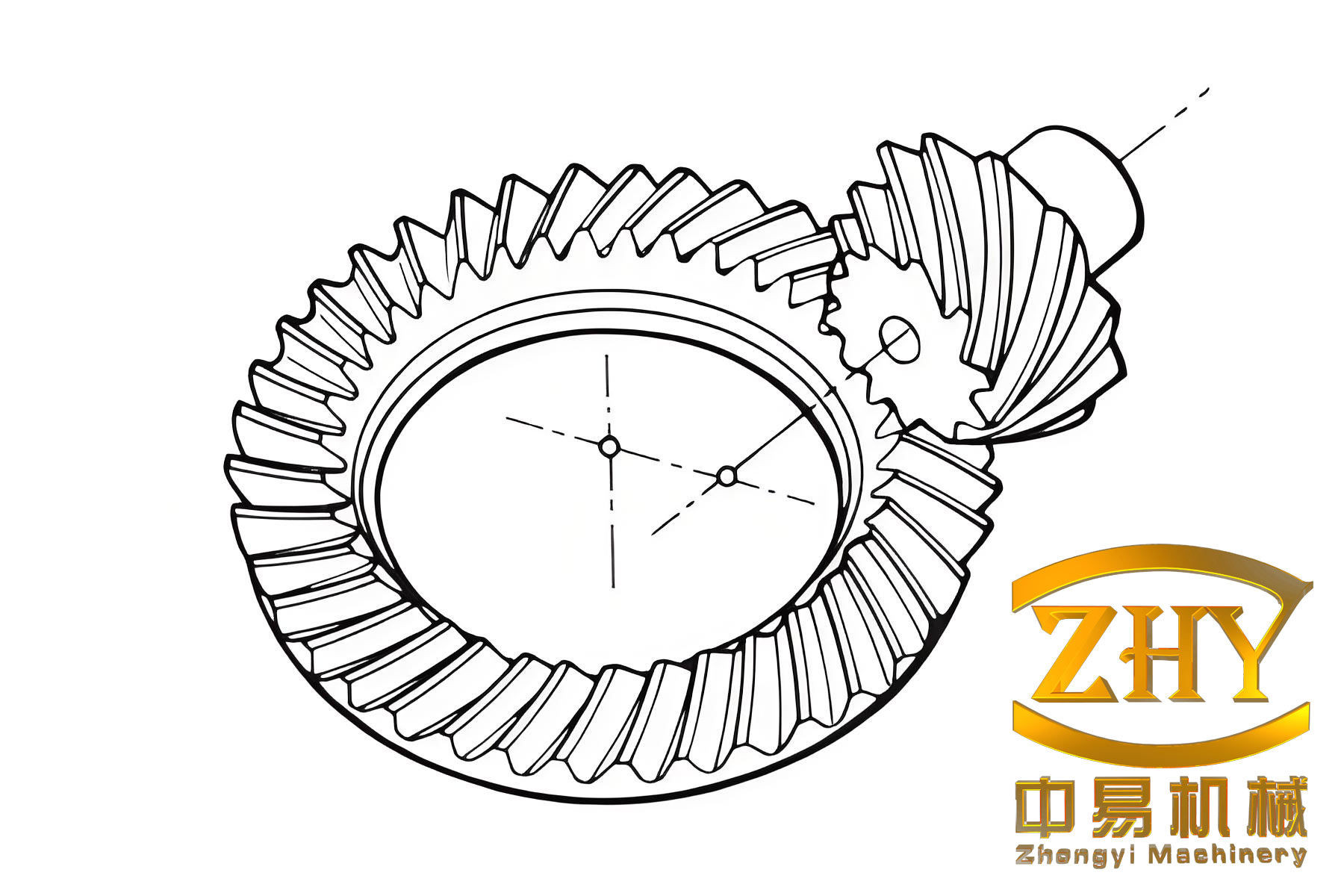
I have studied hypoid bevel gears as critical components in vehicle drive axle main reducers, where their meshing quality, service life, and reliability strongly influence vehicle safety. My work combines differential geometry, gearing theory, tooth contact analysis, finite element modeling, and tool modification design. I focused on establishing an accurate mathematical model of hypoid bevel gears, evaluating their meshing performance under ideal and misaligned conditions, building high-precision finite element models, and improving their performance through cutter blade modification. The entire study was carried out from the perspective of design, manufacturing, and application, and I paid particular attention to the relationship among tooth geometry, contact pattern, transmission error, stress distribution, and modification parameters.
Mathematical Modeling of Hypoid Bevel Gears
I started with the mathematical modeling of hypoid bevel gears. The gear member was assumed to be generated by the formate method, while the pinion member was assumed to be generated by the tilt method. Both members contain a working surface and a transition fillet. I defined the cutter coordinate systems for the gear and pinion separately, and I derived the cutter surface equations and normal equations for the straight cutting edge and the transition fillet. The mathematical model therefore includes not only the working tooth surface but also the root fillet, which is important for bending stress evaluation.
For the gear cutter, the straight cutting edge can be written in the cutter coordinate system as
$$
r_G(s_G,\theta_G)=
\begin{bmatrix}
r_{cG}-s_G\cos\alpha_G\\
(r_{cG}-s_G\sin\alpha_G)\sin\theta_G\\
(r_{cG}-s_G\sin\alpha_G)\cos\theta_G\\
1
\end{bmatrix}
$$
and the corresponding normal vector is
$$
n_G=
\begin{bmatrix}
\sin\alpha_G\\
\cos\alpha_G\sin\theta_G\\
\cos\alpha_G\cos\theta_G
\end{bmatrix}
$$
where \(r_{cG}\) is the cutter tip radius, \(\alpha_G\) is the cutter profile angle, and \(s_G\), \(\theta_G\) are the cutter surface parameters. For the transition fillet, I used a circular arc and transformed it into the gear coordinate system. The gear tooth surface and normal were then obtained by coordinate transformation:
$$
r_2(s_G,\theta_G)=[M_{2B}][M_{BG}]r_G
$$
$$
n_2(s_G,\theta_G)=[L_{2B}][L_{BG}]n_G
$$
For the pinion cutter, the straight cutting edge is expressed as
$$
r_P(s_P,\theta_P)=
\begin{bmatrix}
(r_{cP}+s_P\sin\alpha_P)\cos\theta_P\\
(r_{cP}+s_P\sin\alpha_P)\sin\theta_P\\
-s_P\cos\alpha_P\\
1
\end{bmatrix}
$$
and the normal vector is
$$
n_P=
\begin{bmatrix}
-\cos\alpha_P\cos\theta_P\\
-\cos\alpha_P\sin\theta_P\\
-\sin\alpha_P
\end{bmatrix}
$$
The pinion is generated by a tilt method, so the relative motion between the cutter and the pinion must satisfy the meshing equation. I wrote the cutter surface in the fixed machine coordinate system and imposed
$$
f(s_P,\theta_P,\phi_c)=n_D\cdot v_D^{(c1)}=0
$$
where \(n_D\) is the cutter normal in the fixed coordinate system and \(v_D^{(c1)}\) is the relative velocity between the cutter and the pinion. After solving this equation, the parameter \(s_P\) can be expressed as a function of \(\theta_P\) and \(\phi_c\). The pinion working surface is then obtained by
$$
r_1(\theta_P,\phi_c)=[M_{1F}][M_{FE}][M_{ED}][M_{DC}][M_{CA}][M_{AP}]r_P
$$
$$
n_1(\theta_P,\phi_c)=[L_{1F}][L_{FE}][L_{ED}][L_{DC}][L_{CA}][L_{AP}]n_P
$$
I also derived the transition fillet equations for the pinion in a similar way. The working surface and the transition surface are joined at a boundary. I verified the boundary condition by substituting the boundary parameter into both equations. The coordinates along the tooth height on the working surface and the transition surface were identical, which confirmed that the transition fillet model was consistent with the working surface model.
To visualize the tooth surface and to prepare data for solid modeling, I divided the tooth surface into a grid in the rotating projection plane. Along the tooth width direction, I used
$$
v_{ij}=A_i+\frac{(j-1)(A_o-A_i)}{n-1},\quad i=1,2,\ldots,m,\; j=1,2,\ldots,n
$$
where \(A_i\) and \(A_o\) are the inner and outer cone distances. Along the tooth height direction, I used
$$
h_{ij}=H_j+\frac{(i-1)(H_j’-H_j)}{m-1}
$$
where \(H_j\) and \(H_j’\) are the boundary values on the working surface and the transition surface. By solving the nonlinear tooth surface equations, I obtained the three-dimensional coordinates of all grid points. The pinion concave and convex surfaces were machined separately, so I positioned them using the midpoint chordal height \(h_{m1}\) and the midpoint chordal thickness \(s_{n1}\). The positioning angle \(\theta_x\) was solved from
$$
(x_x\cos\theta_x-y_x\sin\theta_x-x_v)^2+
(y_x\sin\theta_x+z_x\cos\theta_x-z_v)^2=s_{n1}^2
$$
This step ensured that the pinion concave and convex surfaces formed a correct tooth. The basic parameters and machine settings that I used are summarized in the following tables.
| Parameter | Pinion | Gear |
|---|---|---|
| Number of teeth | 8 | 41 |
| Face width / mm | 28.09 | 24.00 |
| Outer cone distance / mm | 97.19 | 84.72 |
| Addendum / mm | 5.77 | 1.02 |
| Dedendum / mm | 2.04 | 6.64 |
| Offset / mm | 23 | |
| Pitch cone angle | 12°32′ | 76°49′ |
| Face cone angle | 17°27′ | 77°44′ |
| Root cone angle | 11°40′ | 71°41′ |
| Design spiral angle | 48°56′ | 30°38′ |
| Cutter fillet radius / mm | 0.65 | 1.00 |
| Midpoint chordal height / mm | 4.80 | 0.83 |
| Midpoint chordal thickness / mm | 6.12 | 3.09 |
| Hand of spiral | LH | RH |
| Gear machine setting | Value |
|---|---|
| Cutter diameter / mm | 152.40 |
| Cutter point width / mm | 1.59 |
| Profile angle / deg | 22.5 |
| Vertical cutter position / mm | 67.7661 |
| Horizontal cutter position / mm | 29.8166 |
| Horizontal wheel position / mm | 0.5984 |
| Wheel mounting angle / deg | 70.88 |
| Pinion machine setting | Concave side | Convex side |
|---|---|---|
| Cutter diameter / mm | 161.04 | 149.86 |
| Cutter point width / mm | 0 | 0 |
| Profile angle / deg | 20.0 | 25.0 |
| Radial cutter position / mm | 73.9536 | 72.5171 |
| Tilt angle / deg | 16.73 | 19.17 |
| Cutter rotation angle / deg | 346.66 | 337.92 |
| Vertical wheel position / mm | 19.6316 | 23.0267 |
| Horizontal wheel position / mm | 2.3949 | -1.7553 |
| Bed position / mm | 2.6682 | 7.7363 |
| Wheel mounting angle / deg | 358.01 | 355.16 |
| Roll ratio | 5.064418 | 4.816942 |
| Angular cutter position / deg | 83.61 | 77.42 |
I used both cutting simulation and reverse modeling to build solid models of the hypoid bevel gears. In the cutting simulation method, I modeled the cutter and the blank, assembled them according to the machine settings, and then performed Boolean operations to remove material. For the gear, the cutter was fixed and the blank was indexed after each tooth slot. For the pinion, the generating motion was divided into many small steps, and the cutter and blank were rotated according to the roll ratio. This approach produced a high-precision solid model. In the reverse modeling method, I exported the tooth surface point cloud from my mathematical model, imported it into a three-dimensional CAD environment, and reconstructed the tooth surface by surface fitting. I then compared the reconstructed surfaces with the original point cloud. The deviations showed that the cutting simulation method gave smaller errors for both the gear and the pinion. This result also verified the accuracy of my mathematical model of hypoid bevel gears.
| Surface | Method | Gear deviation / mm | Pinion deviation / mm |
|---|---|---|---|
| Convex | Cutting simulation | 0.007–0.036 | 0.000–0.024 |
| Convex | Reverse modeling | 0.035–0.124 | 0.000–0.098 |
| Concave | Cutting simulation | 0.024–0.065 | 0.017–0.030 |
| Concave | Reverse modeling | 0.045–0.171 | 0.062–0.116 |
Tooth Contact Analysis of Hypoid Bevel Gears
After building the mathematical model, I studied the tooth contact analysis of hypoid bevel gears. I used both the theoretical TCA method and the Ease-off-TCA method. In the theoretical TCA method, the two tooth surfaces must have the same position vector and the same normal vector at the instantaneous contact point in the fixed coordinate system. Therefore, I solved
$$
r_h^{(1)}(\theta_P,\phi_c,\phi_1)=r_h^{(2)}(s_G,\theta_G,\phi_2)
$$
$$
n_h^{(1)}(\theta_P,\phi_c,\phi_1)=n_h^{(2)}(s_G,\theta_G,\phi_2)
$$
These vector equations give five independent scalar equations. By fixing the pinion rotation angle \(\phi_1\) and solving for the remaining five unknowns, I obtained one contact point. Repeating this process for a sequence of \(\phi_1\) values produced the contact path. At the reference point, the instantaneous transmission ratio must equal the nominal gear ratio. The instantaneous transmission ratio can be written as
$$
i(t)=\frac{(p_2\times R_2)\cdot n_2}{(p_1\times R_1)\cdot n_1}
$$
where \(p_2=(0,0,1)^T\), \(p_1=(-1,0,0)^T\), and \(R_1\), \(R_2\) are the position vectors of the two contacting surfaces. The transmission error of hypoid bevel gears is defined as
$$
\Delta\phi_2=
(\phi_2-\phi_2^{(0)})-
\frac{Z_1}{Z_2}(\phi_1-\phi_1^{(0)})
$$
where \(Z_1\) and \(Z_2\) are the numbers of teeth of the pinion and gear, and \(\phi_1^{(0)}\), \(\phi_2^{(0)}\) are the initial meshing angles at the reference point.
Because hypoid bevel gears are in point contact, the actual contact region is an ellipse due to elastic deformation. I calculated the contact ellipse by using the principal curvatures and principal directions of the two mating surfaces. The semi-major axis \(a\) and semi-minor axis \(b\) are
$$
a=\sqrt{\frac{\epsilon}{A}},\qquad
b=\sqrt{\frac{\epsilon}{B}}
$$
where \(\epsilon\) is the elastic deformation, usually taken as \(0.00635\) mm for gear steels, and
$$
A=\frac{1}{4}\left[
K_1-K_2-
\sqrt{(g_1-g_2)^2+4g_1g_2\cos2\alpha^{(12)}}
\right]
$$
$$
B=\frac{1}{4}\left[
K_1+K_2-
\sqrt{(g_1-g_2)^2+4g_1g_2\cos2\alpha^{(12)}}
\right]
$$
The angle \(\alpha^{(1)}\) between the principal direction of the pinion and the minor axis of the contact ellipse is obtained from
$$
\tan\alpha^{(1)}=
\frac{T}{1+T}
$$
with
$$
T=
\frac{
g_1-g_2+
\sqrt{(g_1-g_2)^2+4g_1g_2\cos2\alpha^{(12)}}
}{
2g_1g_2\sin2\alpha^{(12)}
}
$$
The Ease-off-TCA method is based on the conjugate tooth surface of the pinion. I treated the gear tooth surface as a virtual cutter and generated an auxiliary pinion surface that is fully conjugate to the gear. The auxiliary pinion surface and its normal are
$$
r_1^{(0)}(\theta_G,\phi_1,\phi_2)=[M_{1h}][M_{h2}]r_2(s_G,\theta_G)
$$
$$
n_1^{(0)}(\theta_G,\phi_1,\phi_2)=[L_{1h}][L_{h2}]n_2(s_G,\theta_G)
$$
and the meshing condition is
$$
f(s_G,\theta_G,\phi_1,\phi_2)=0
$$
At a given pinion rotation angle, the auxiliary pinion surface has an instantaneous conjugate meshing line. I discretized this line and projected it onto the rotating projection plane. For each discrete point, I calculated the distance between the auxiliary surface point and the corresponding point on the theoretical pinion surface:
$$
H(j)=
\sqrt{
(x_1(j)-x_0(j))^2+
(y_1(j)-y_0(j))^2+
(z_1(j)-z_0(j))^2
}
$$
The minimum distance at the \(i\)-th pinion angle is the transmission error:
$$
\Delta\epsilon^{(i)}=\min_j H(j)
$$
and the corresponding point is the meshing point. The angular transmission error can be obtained by
$$
\Delta Te^{(i)}=
\frac{Z_2}{Z_1}
\frac{\Delta\epsilon^{(i)}}{z_1 n_y-y_1 n_z}
$$
I compared the theoretical TCA and Ease-off-TCA results for hypoid bevel gears. The contact patterns and transmission error curves were almost identical when no assembly error was applied and when assembly errors were applied. This validated the accuracy and feasibility of the Ease-off-TCA method. The advantage of Ease-off-TCA is that it reduces the number of nonlinear equations, avoids the calculation of principal curvatures and principal directions for the contact ellipse, and can handle edge contact more naturally. Therefore, I used Ease-off-TCA for the subsequent installation error analysis and modification evaluation.
I analyzed the influence of installation errors on the meshing performance of hypoid bevel gears. The main installation errors considered were the pinion mounting distance error \(e_H\), the gear mounting distance error \(e_V\), the shaft center distance error \(e_{os}\), and the shaft angle error \(e_\Sigma\). The results showed a regular relationship between the contact area and the installation errors. The pinion mounting distance error mainly moved the contact area along the tooth height direction. The gear mounting distance error mainly moved the contact area along the tooth width direction. The shaft center distance error and the shaft angle error also mainly changed the contact position along the tooth height direction. When multiple installation errors act together, the contact area movement depends on the signs and directions of the individual errors.
| Contact position | \(e_V\) / mm | \(e_H\) / mm |
|---|---|---|
| \(b/4\) | 0.2596 | -0.1740 |
| \(b/2\) | -0.2624 | 0.0675 |
| \(3b/4\) | -0.9057 | 0.3839 |
| No error | 0 | 0 |
When \(e_{os}\) and \(e_\Sigma\) had the same sign, the contact area movement along the tooth width direction was enhanced. When they had opposite signs, the contact area movement along the tooth height direction was enhanced. These results are useful for predicting the actual contact pattern of hypoid bevel gears under assembly errors.
Finite Element Modeling and Stress Analysis of Hypoid Bevel Gears
I developed a method for automatic finite element mesh generation and precise finite element model assembly for hypoid bevel gears. Instead of importing a solid model into finite element software and manually meshing it, I generated the finite element mesh directly from the mathematical tooth surface equations. I divided the working surface, transition surface, fillet connection, and wheel body into a structured grid. The mesh density could be controlled independently in the tooth height, tooth width, tooth thickness, and body height directions. This approach avoided short edges, broken surfaces, and other defects that often appear during solid-model meshing.
For the working surface mesh, I projected the tooth surface points onto the rotating projection plane. The projection and rotation matrices are
$$
M_1=
\begin{bmatrix}
\cos\Gamma & \sin\Gamma\\
-\sin\Gamma & \cos\Gamma
\end{bmatrix}
$$
$$
\begin{bmatrix}
A_x\\
A_y
\end{bmatrix}
=
M_1
\begin{bmatrix}
A_x\\
\sqrt{A_y^2+A_z^2}
\end{bmatrix}
$$
The angular difference between two corresponding points \(A\) and \(B\) on the concave and convex surfaces is
$$
\theta_K=
\cos^{-1}
\left(
\frac{y_Ay_B+z_Az_B}
{\sqrt{y_A^2+z_A^2}\sqrt{y_B^2+z_B^2}}
\right)
$$
I divided this angle into \((M_S-1)\) equal parts and rotated the points incrementally. The rotation matrix for the \(i\)-th subdivision is
$$
M_K=
\begin{bmatrix}
1 & 0 & 0\\
0 & \cos\left(\frac{D_n(i-1)\theta_K}{M_S-1}\right) & \sin\left(\frac{D_n(i-1)\theta_K}{M_S-1}\right)\\
0 & -\sin\left(\frac{D_n(i-1)\theta_K}{M_S-1}\right) & \cos\left(\frac{D_n(i-1)\theta_K}{M_S-1}\right)
\end{bmatrix}
$$
where \(D_n=-1\) for a left-hand gear and \(D_n=1\) for a right-hand gear. The final coordinates of the finite element nodes on the working surface were obtained by
$$
x_i=t_x\cos\theta_J,\qquad
y_i=t_y\sin\theta_J,\qquad
z_i=-t_y\cos\theta_J
$$
where \(\theta_J\) is the angular position of the rotated point. A similar procedure was used for the transition surface and the wheel body. The eight-node linear reduced-integration element C3D8R was selected for the finite element analysis because it performs well under contact and bending conditions when the mesh is sufficiently fine. The node ordering for a typical hexahedral element is given in the following table.
| Node label | Node number |
|---|---|
| a | a |
| b | a + MW |
| c | a + MW × MS |
| d | a + MW × MS + MW |
| e | a + 1 |
| f | a + MW + 1 |
| g | a + MW × MS + 1 |
| h | a + MW × MS + MW + 1 |
For the finite element model assembly, I used the TCA results to determine the meshing angles of the pinion and gear at each contact point. The node coordinates of the pinion and gear were transformed into the fixed coordinate system by using the corresponding rotation angles. In this way, the pinion and gear could be assembled precisely at any contact position along the contact path without manual adjustment. This method eliminated interference and gaps that often occur in manual assembly and improved the accuracy of the finite element analysis of hypoid bevel gears.
I wrote the finite element model data, material properties, contact definitions, analysis steps, loads, and boundary conditions into an ABAQUS input file. The input file was then submitted to a batch-processing tool, which allowed multiple contact positions to be analyzed sequentially without repeated manual operations. This significantly reduced the repetitive workload and improved the analysis efficiency for hypoid bevel gears.
The mesh parameters that I used were as follows: working surface divisions along tooth height \(M_I=20\), transition surface divisions along tooth height \(M_{II}=10\), tooth width divisions \(M_W=40\), wheel body height divisions \(M_{III}=5\), tooth thickness divisions \(M_S=7\), fillet connection divisions \(M_C=2\), and wheel body projection height \(L=12\). The resulting finite element models of the gear and pinion each contained 48,200 nodes and 39,624 elements.
| Mesh parameter | Value |
|---|---|
| Working surface divisions along tooth height \(M_I\) | 20 |
| Transition surface divisions along tooth height \(M_{II}\) | 10 |
| Tooth width divisions \(M_W\) | 40 |
| Wheel body height divisions \(M_{III}\) | 5 |
| Tooth thickness divisions \(M_S\) | 7 |
| Fillet connection divisions \(M_C\) | 2 |
| Wheel body projection height \(L\) / mm | 12 |
| Nodes per member | 48,200 |
| Elements per member | 39,624 |
I carried out static finite element analysis of hypoid bevel gears under different loads and installation errors. The material properties were assigned as follows: elastic modulus \(206000\) MPa, Poisson ratio \(0.3\), and density \(7.8\times10^{-9}\) kg/mm\(^3\). The gear was loaded with a torque about its axis, and the pinion was fixed except for its rotation about its own axis. The contact between the gear convex surface and the pinion concave surface was defined as a surface-to-surface contact pair.
The stress analysis showed that the contact region was elliptical, which agreed with the theoretical contact ellipse. The maximum contact stress occurred near the center of the contact ellipse, and the stress decreased gradually toward the edge. During the meshing cycle, the hypoid bevel gears experienced multi-tooth contact, single-tooth contact, and multi-tooth contact again. This behavior was reflected in the stress curves. Under a torque of \(500\) N·m, the maximum root bending stress of the gear was \(200.294\) MPa, and that of the pinion was \(190.024\) MPa. The maximum contact stress of the gear was \(1260.05\) MPa, and that of the pinion was \(1217.3\) MPa. The gear experienced higher contact stress than the pinion throughout the meshing cycle.
| Load / N·m | Gear max root bending stress / MPa | Pinion max root bending stress / MPa | Gear max contact stress / MPa | Pinion max contact stress / MPa |
|---|---|---|---|---|
| 200 | 90.0117 | 90.1404 | 982.4 | 882.825 |
| 350 | 154.607 | 144.48 | 1089 | 1004 |
| 500 | 200.294 | 190.024 | 1260.05 | 1217.3 |
I also studied the influence of installation errors on the strength of hypoid bevel gears. By adjusting \(e_V\) and \(e_H\), I forced the contact to occur at the toe, the middle, and the heel of the tooth. Under a torque of \(500\) N·m, the maximum root bending stress and contact stress were highest when contact occurred near the toe. The stresses were lowest when contact occurred near the middle of the tooth. This result indicates that, in practical assembly, the contact pattern should be kept near the middle of the tooth to reduce the risk of fatigue failure and to improve the reliability of hypoid bevel gears.
| Contact position | Gear max root bending stress / MPa | Pinion max root bending stress / MPa | Gear max contact stress / MPa | Pinion max contact stress / MPa |
|---|---|---|---|---|
| Toe | Highest | Highest | Highest | Highest |
| Middle | Lowest | Lowest | Lowest | Lowest |
| Heel | Intermediate | Intermediate | Intermediate | Intermediate |
I also performed modal analysis of the hypoid bevel gears. The first ten natural frequencies of the gear and pinion were extracted. The results showed that the pinion natural frequencies changed more widely than the gear natural frequencies over the first ten modes. When resonance occurs, the pinion mainly exhibits torsional distortion of the teeth along the circumference, while the gear exhibits distortion both along the circumference and along the axial direction. These frequencies should be avoided in the design and operation of hypoid bevel gears.
| Mode | Gear natural frequency / Hz | Pinion natural frequency / Hz |
|---|---|---|
| 1 | 20177 | 23013 |
| 2 | 20260 | 23020 |
| 3 | 20268 | 32110 |
| 4 | 20558 | 48069 |
| 5 | 20564 | 50977 |
| 6 | 21178 | 50988 |
| 7 | 21186 | 61376 |
| 8 | 22269 | 61381 |
| 9 | 22272 | 68757 |
| 10 | 23933 | 69165 |
Modification Design and Optimization of Hypoid Bevel Gears
To further improve the performance of hypoid bevel gears, I replaced the straight cutting edge of the pinion cutter with curved cutting edges. I designed both a second-order parabolic blade and a fourth-order parabolic blade. The gear cutter remained a straight-edge cutter. By changing the blade shape, the pinion tooth surface could be modified without changing the machine settings extensively. This approach is simpler and easier to implement than changing the roll ratio or using complex NURBS surface fitting.
For the second-order parabolic blade, the cutting edge was divided into a parabolic portion and a circular fillet portion. The parabolic portion can be written as
$$
r_a=
\begin{bmatrix}
[r_{cP}+s_P\sin\alpha_P\mp T\cos\alpha_P]\cos\theta_P\\
[r_{cP}+s_P\sin\alpha_P\mp T\cos\alpha_P]\sin\theta_P\\
-s_P\cos\alpha_P\pm T\sin\alpha_P\\
1
\end{bmatrix}
$$
where
$$
T=a_1(s_P-A_0)^2
$$
The normal vector of the parabolic portion is
$$
n_a=
\begin{bmatrix}
[\cos\alpha_P\mp 2a_1(s_P-A_0)\sin\alpha_P]\cos\theta_P\\
[\cos\alpha_P\mp 2a_1(s_P-A_0)\sin\alpha_P]\sin\theta_P\\
-\sin\alpha_P\pm 2a_1(s_P-A_0)\cos\alpha_P
\end{bmatrix}
\Big/
\sqrt{1+4a_1^2(s_P-A_0)^2}
$$
The circular fillet portion is described by
$$
r_b=
\begin{bmatrix}
x_f\pm(r_f\cos\theta_f)\\
(r_f\cos\theta_f)\cos\theta_P\\
(r_f\cos\theta_f)\sin\theta_P\\
(1-\sin\theta_f)r_f
\end{bmatrix}
$$
and its normal vector is
$$
n_b=
\begin{bmatrix}
\mp\cos\theta_f\cos\theta_P\\
\mp\cos\theta_f\sin\theta_P\\
-\sin\theta_f
\end{bmatrix}
$$
At the junction point, the normal vectors of the parabolic portion and the circular fillet portion must be equal. This condition determines the fillet radius \(r_f\) and the junction point position.
For the fourth-order parabolic blade, the parabolic portion is replaced by a fourth-order curve:
$$
T=b_1(s_P-B_0)^4+b_2(s_P-B_0)^2
$$
The cutting edge and normal vector have the same form as the second-order case, but the derivative \(dT/ds_P\) becomes
$$
\frac{dT}{ds_P}=4b_1(s_P-B_0)^3+2b_2(s_P-B_0)
$$
In my calculations, I set \(b_2=0\) to simplify the study, because the second-order term mainly introduces behavior similar to the second-order parabolic blade. The fourth-order term allows a higher-order transmission error curve, which can make the meshing motion smoother.
I used a multi-objective optimization model to determine the cutter parameters. The optimization objectives were the transmission error, the position symmetry, and the coincidence degree. The position symmetry was defined as the ratio of the time from meshing-in to the reference point and the time from the reference point to meshing-out. The coincidence degree was defined as
$$
C_r=\frac{T_c}{T_z}
$$
where \(T_c\) is the pinion rotation angle from the beginning of meshing to the end of meshing for one tooth pair, and \(T_z=2\pi/Z_1\) is one meshing cycle. For the second-order parabolic blade, the optimization model was
$$
\min \Delta\phi_2(a_1,A_0)
$$
$$
\text{subject to}\quad
\zeta(a_1,A_0)=B,\qquad
C_r(a_1,A_0)=C
$$
where \(a_1\) and \(A_0\) are the design variables. For the fourth-order parabolic blade, the optimization model was
$$
\min \Delta\phi_2(b_1,b_2,B_0)
$$
$$
\text{subject to}\quad
\zeta(b_1,b_2,B_0)=E,\qquad
C_r(b_1,b_2,B_0)=F
$$
I solved these optimization problems with the NSGA2 algorithm. The crowding distance used in NSGA2 is
$$
d_i=
\sum_{m=1}^{M}
\frac{
|f_m(i+1)-f_m(i-1)|
}{
f_m^{\max}-f_m^{\min}
}
$$
The algorithm uses non-dominated sorting, crowding distance comparison, tournament selection, crossover, and mutation. I set the population size to 50, the maximum number of generations to 100, the crossover probability to 0.7, the mutation percentage to 0.4, and the mutation rate to 0.02. The optimization results are summarized in the following tables.
| Coincidence degree | Symmetry | Transmission error / arcsec | \(a_1\) | \(A_0\) |
|---|---|---|---|---|
| 1.5 | 1.0 | 41.3075 | \(9.7105\times10^{-4}\) | 3.2316 |
| 1.5 | 1.2 | 43.2603 | \(1.1000\times10^{-3}\) | 3.5487 |
| 1.8 | 1.0 | 76.9100 | \(2.0000\times10^{-3}\) | 3.3571 |
| 1.8 | 1.2 | 83.3975 | \(2.2000\times10^{-3}\) | 3.4514 |
| Coincidence degree | Symmetry | Transmission error / arcsec | \(b_1\) | \(B_0\) |
|---|---|---|---|---|
| 1.5 | 1.0 | 36.2953 | \(9.9144\times10^{-5}\) | 3.4967 |
| 1.5 | 1.2 | 40.5263 | \(7.8481\times10^{-5}\) | 3.7723 |
| 1.8 | 1.0 | 68.9701 | \(2.3933\times10^{-4}\) | 3.3204 |
| 1.8 | 1.2 | 76.1421 | \(2.0590\times10^{-4}\) | 3.4945 |
I also studied how the transmission error affects the stress of hypoid bevel gears. I preset maximum transmission error amplitudes of \(25\) arcsec, \(50\) arcsec, and \(100\) arcsec, and then solved for the corresponding cutter parameters. The finite element results showed that the transmission error mainly affects the maximum contact stress. As the transmission error increased, the maximum contact stress of both the gear and the pinion increased. The maximum root bending stress, however, remained almost unchanged. The gear and pinion also showed larger stress fluctuations during meshing-in and meshing-out when the transmission error was larger. These results are useful for balancing transmission error, contact stress, and bending stress in the modification design of hypoid bevel gears.
| Maximum transmission error / arcsec | Gear max contact stress trend | Pinion max contact stress trend | Gear max root bending stress trend | Pinion max root bending stress trend |
|---|---|---|---|---|
| 25 | Lowest | Lowest | Nearly unchanged | Nearly unchanged |
| 50 | Medium | Medium | Nearly unchanged | Nearly unchanged |
| 100 | Highest | Highest | Nearly unchanged | Nearly unchanged |
Summary of Results for Hypoid Bevel Gears
I established a complete mathematical model of hypoid bevel gears with transition fillets, including the gear working surface, gear transition surface, pinion working surface, and pinion transition surface. The boundary conditions between the working surface and the transition surface were verified, and the tooth surfaces were visualized by numerical simulation. I used the midpoint chordal height and midpoint chordal thickness to position the pinion concave and convex surfaces accurately. The cutting simulation method produced solid models with smaller deviations than the reverse modeling method, which confirmed the accuracy of my mathematical model and the feasibility of the cutting simulation approach.
I studied the tooth contact analysis of hypoid bevel gears with both theoretical TCA and Ease-off-TCA. The two methods gave nearly identical contact patterns and transmission error curves under both ideal and misaligned conditions. Ease-off-TCA reduced the number of nonlinear equations and avoided the complex calculation of principal curvatures and directions, so it was more concise and efficient. I analyzed the influence of installation errors on the contact pattern. The pinion mounting distance error, shaft center distance error, and shaft angle error mainly affected the contact position along the tooth height direction. The gear mounting distance error mainly affected the contact position along the tooth width direction. When multiple errors acted together, the resulting contact pattern could be predicted from the signs and directions of the individual errors.
I developed an automatic finite element mesh generation method and a precise assembly method for hypoid bevel gears. The finite element model was generated directly from the mathematical tooth surface equations, which avoided the defects caused by solid-model meshing. The pinion and gear were assembled at each contact position by using the TCA results. The ABAQUS input file and batch processing allowed multiple contact positions to be analyzed efficiently. The finite element results showed that the gear experienced higher root bending stress and contact stress than the pinion. Under installation errors, the stresses were highest when contact occurred near the toe and lowest when contact occurred near the middle of the tooth. The modal analysis provided the first ten natural frequencies of the gear and pinion, which can be used to avoid resonance in hypoid bevel gear systems.
I designed second-order and fourth-order parabolic cutting blades for the pinion of hypoid bevel gears. The blade equations and normal equations were derived, and the fillet geometry was determined by the normal continuity condition at the junction point. I used NSGA2 multi-objective optimization to obtain the cutter parameters that satisfied the desired position symmetry and coincidence degree while minimizing the transmission error. The fourth-order parabolic blade produced smaller transmission error than the second-order blade under the same constraints and allowed a higher-order transmission error curve. The stress analysis showed that transmission error mainly affects the maximum contact stress, while the maximum root bending stress is almost unchanged. These findings provide a useful reference for the design, manufacturing, and application of high-performance hypoid bevel gears.