
In modern equipment manufacturing, gears are among the most critical basic components, and their machining accuracy directly determines the performance, reliability, and service life of automotive, aerospace, and industrial transmission systems. Among the various gear manufacturing methods, gear hobbing is one of the most widely used processes because of its high efficiency, strong adaptability, and ability to produce both spur and helical gears. However, the quality of gear hobbing is affected by many coupled factors, including process parameters, design parameters, tool conditions, machine tool states, environmental disturbances, and measurement uncertainties. These factors make the analysis of gear hobbing quality and the prediction of gear errors a challenging problem. In this study, I focus on the analysis of factors affecting gear hobbing quality and the development of a quality prediction method. The research integrates correlation analysis, density peak clustering, improved multi-threshold Birch clustering, fuzzy rough set theory, multi-objective differential evolution, and improved variational inference Gaussian mixture regression. The goal is to extract low-dimensional quality inspection indicators that reflect the true machining quality of gears, reduce the process parameters to a set of characteristic parameters, quantify their importance, and establish an accurate and robust prediction model for gear hobbing quality.
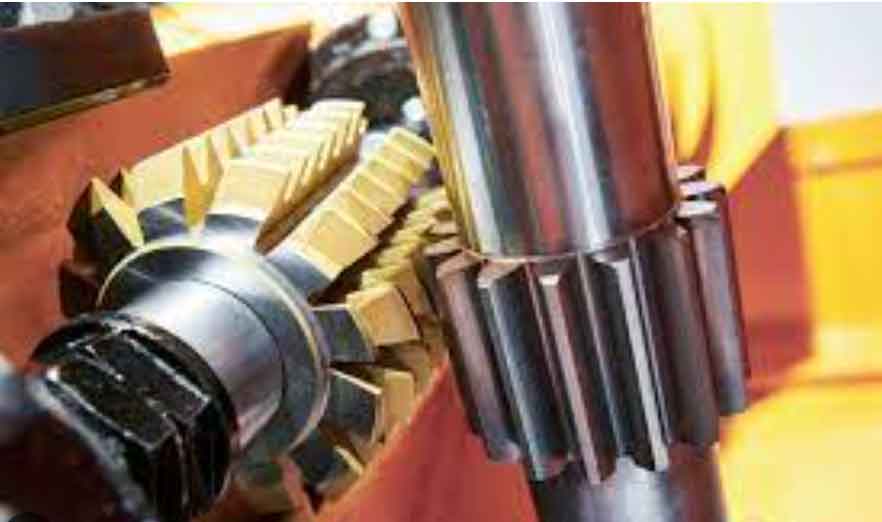
In a typical gear hobbing process, the hob and the workpiece rotate in a coordinated manner while the hob feeds along the axial direction of the workpiece. The cutting motion is generated by the relative movement between the hob and the gear blank. The process is illustrated below.
The quality of a hobbed gear is usually evaluated by a large number of inspection indicators, such as single pitch deviation, cumulative pitch deviation, profile total deviation, helix deviation, runout, and many others. These indicators are often highly correlated and contain redundant information. If all of them are used for quality analysis and prediction, the computational cost increases dramatically, and the analysis efficiency decreases. Moreover, the process parameters and design parameters contain a large amount of hidden information. Without a systematic reduction method, it is difficult to determine which parameters have the greatest influence on gear hobbing quality. Therefore, I propose a systematic framework that first analyzes the internal relationships among quality inspection indicators, then reduces the process and design parameters, and finally builds a quality prediction model based on the reduced parameters.
The remainder of this article is organized as follows. First, I describe the data collection and preprocessing for gear hobbing. Second, I present the quality inspection indicator analysis method based on density peak clustering and improved multi-threshold Birch clustering. Third, I introduce the process parameter reduction method based on fuzzy rough set theory and an improved multi-objective differential evolution algorithm. Fourth, I develop the gear hobbing quality prediction model using improved variational inference Gaussian mixture regression. Finally, I demonstrate the effectiveness of the proposed methods through a case study and provide conclusions.
Data Description and Preprocessing
In this research, the gear hobbing process involves three main types of parameters: gear quality inspection indicators, gear design parameters, and gear process parameters. The gear design parameters and process parameters are treated as input variables, while the quality inspection indicators are treated as output variables. Let the gear design parameters be denoted by
$$ X_{de}^{(D)} = \{x_{de}^{1}, x_{de}^{2}, \ldots, x_{de}^{D}\} $$
and the gear process parameters be denoted by
$$ X_{pr}^{(P)} = \{x_{pr}^{1}, x_{pr}^{2}, \ldots, x_{pr}^{P}\} $$
where \(D\) and \(P\) are the dimensions of the design and process parameter sets, respectively. The union of the design and process parameters is called the gear parameter set:
$$ X_{gp}^{(r)} = X_{de}^{(D)} \cup X_{pr}^{(P)} $$
where \(r = D + P\). In this study, the quality inspection indicators are denoted by
$$ Y_{qua}^{(L)} = \{y_{qua}^{1}, y_{qua}^{2}, \ldots, y_{qua}^{L}\} $$
where \(L\) is the number of quality inspection indicators. For the gear hobbing case considered here, \(L = 44\). The quality inspection indicators include cross-ball dimension, single pitch deviation, adjacent pitch deviation, cumulative pitch deviation, runout, profile tilt, profile total deviation, profile form deviation, profile crowning, helix tilt, helix total deviation, helix form deviation, helix crowning, and their corresponding standard deviations on both flanks. The detailed definitions follow international gear accuracy standards.
Because the parameters have different units and scales, I apply Z-score standardization to the gear parameter set before analysis. The standardization formula is
$$ x_{gp}^{i} = \frac{x_{gp}^{i} – \mu_{gp}}{\sigma_{gp}} $$
where \(x_{gp}^{i}\) is the original value, \(\mu_{gp}\) is the mean, and \(\sigma_{gp}\) is the standard deviation. The same standardization is applied to the quality inspection data. This preprocessing step avoids the influence of different dimensions and improves the convergence speed and accuracy of the subsequent models.
Table 1 lists the gear process parameters considered in this study. Table 2 lists the gear design parameters. Table 3 lists the quality inspection parameters. These tables provide the basic notation used throughout the article.
| No. | Symbol | Name | Unit |
|---|---|---|---|
| 1 | \(V\) | Spindle speed | r/min |
| 2 | \(V_f\) | Feed speed | m/min |
| 3 | \(T_c\) | Tool coating material | HV0.05 |
| 4 | \(N_t\) | Number of hob starts | — |
| 5 | \(W_f\) | Cold air wind speed | m/s |
| 6 | \(\alpha_p\) | Cutting depth | mm |
| No. | Symbol | Name | Unit |
|---|---|---|---|
| 1 | \(m\) | Module | mm |
| 2 | \(\alpha\) | Pressure angle | deg |
| 3 | \(\beta\) | Helix angle | deg |
| 4 | \(d_b\) | Base circle diameter | mm |
| 5 | \(b\) | Face width | mm |
| 6 | \(d_a\) | Tip circle diameter | mm |
| 7 | \(Z\) | Number of teeth | — |
| 8 | \(x_m\) | Profile shift coefficient | mm |
| No. | Symbol | Name | No. | Symbol | Name |
|---|---|---|---|---|---|
| 1 | \(M_e\) | Cross-ball dimension | 23 | \(ff_{\alpha dL}\) | Profile form deviation std. dev. (left) |
| 2 | \(f_{ptL}\) | Single pitch deviation (left) | 24 | \(ff_{\alpha dR}\) | Profile form deviation std. dev. (right) |
| 3 | \(f_{ptR}\) | Single pitch deviation (right) | 25 | \(C_{\alpha mL}\) | Profile crowning mean (left) |
| 4 | \(f_{uL}\) | Adjacent pitch deviation (left) | 26 | \(C_{\alpha mR}\) | Profile crowning mean (right) |
| 5 | \(f_{uR}\) | Adjacent pitch deviation (right) | 27 | \(C_{\alpha dL}\) | Profile crowning std. dev. (left) |
| 6 | \(R_{pL}\) | Pitch deviation (left) | 28 | \(C_{\alpha dR}\) | Profile crowning std. dev. (right) |
| 7 | \(R_{pR}\) | Pitch deviation (right) | 29 | \(f_{H\beta mL}\) | Helix tilt mean (left) |
| 8 | \(F_{pL}\) | Total cumulative pitch deviation (left) | 30 | \(f_{H\beta mR}\) | Helix tilt mean (right) |
| 9 | \(F_{pR}\) | Total cumulative pitch deviation (right) | 31 | \(f_{H\beta dL}\) | Helix tilt std. dev. (left) |
| 10 | \(F_{piL}\) | Single-tooth cumulative pitch deviation (left) | 32 | \(f_{H\beta dR}\) | Helix tilt std. dev. (right) |
| 11 | \(F_{piR}\) | Single-tooth cumulative pitch deviation (right) | 33 | \(F_{\beta mL}\) | Helix total deviation mean (left) |
| 12 | \(F_r\) | Radial runout | 34 | \(F_{\beta mR}\) | Helix total deviation mean (right) |
| 13 | \(f_{H\alpha mL}\) | Profile tilt mean (left) | 35 | \(F_{\beta dL}\) | Helix total deviation std. dev. (left) |
| 14 | \(f_{H\alpha mR}\) | Profile tilt mean (right) | 36 | \(F_{\beta dR}\) | Helix total deviation std. dev. (right) |
| 15 | \(f_{H\alpha dL}\) | Profile tilt std. dev. (left) | 37 | \(ff_{\beta mL}\) | Helix form deviation mean (left) |
| 16 | \(f_{H\alpha dR}\) | Profile tilt std. dev. (right) | 38 | \(ff_{\beta mR}\) | Helix form deviation mean (right) |
| 17 | \(F_{\alpha mL}\) | Profile total deviation mean (left) | 39 | \(ff_{\beta dL}\) | Helix form deviation std. dev. (left) |
| 18 | \(F_{\alpha mR}\) | Profile total deviation mean (right) | 40 | \(ff_{\beta dR}\) | Helix form deviation std. dev. (right) |
| 19 | \(F_{\alpha dL}\) | Profile total deviation std. dev. (left) | 41 | \(C_{\beta mL}\) | Helix crowning mean (left) |
| 20 | \(F_{\alpha dR}\) | Profile total deviation std. dev. (right) | 42 | \(C_{\beta mR}\) | Helix crowning mean (right) |
| 21 | \(ff_{\alpha mL}\) | Profile form deviation mean (left) | 43 | \(C_{\beta dL}\) | Helix crowning std. dev. (left) |
| 22 | \(ff_{\alpha mR}\) | Profile form deviation mean (right) | 44 | \(C_{\beta dR}\) | Helix crowning std. dev. (right) |
Quality Inspection Indicator Analysis
The quality inspection indicators in gear hobbing are numerous and often exhibit strong internal correlations. If all indicators are used simultaneously, the analysis becomes inefficient, and some important but less numerous indicators may be masked by others. Therefore, I propose a method to extract a set of relatively independent low-dimensional quality inspection indicators that can comprehensively reflect the actual gear hobbing quality. The method consists of three steps: correlation analysis, density peak clustering (DPCA), and improved multi-threshold Birch clustering (IBirch).
First, I compute the correlation between every pair of quality inspection indicators. Three correlation coefficients are considered: Pearson product-moment correlation, Kendall rank correlation, and Spearman rank correlation. The Pearson correlation coefficient between two indicators \(X\) and \(Y\) is
$$ r = \frac{\sum (X – \bar{X})(Y – \bar{Y})}{\sqrt{\sum (X – \bar{X})^2 \sum (Y – \bar{Y})^2}} $$
The Kendall rank correlation is
$$ r = \frac{\sum_{i=1}^{n-1} \sum_{j=i+1}^{n} \operatorname{sgn}(X_i – X_j)\operatorname{sgn}(Y_i – Y_j)}{n(n-1)} $$
The Spearman rank correlation is
$$ r = 1 – \frac{6 \sum_{i=1}^{n} (P_i – Q_i)^2}{n(n^2 – 1)} $$
where \(P_i\) and \(Q_i\) are the ranks of the two variables. Based on these coefficients, I obtain a correlation matrix for all quality inspection indicators. The correlation matrix reveals which indicators are strongly related and which are relatively independent.
Second, I apply density peak clustering to the correlation matrix. For each quality inspection indicator \(i\), I compute a local density \(\rho_i\) and a distance \(\delta_i\). The local density is defined as
$$ \rho_i = \sum_j \chi(d_{ij} – d_c) $$
where \(d_{ij}\) is the distance between indicator \(i\) and indicator \(j\), \(d_c\) is a cutoff distance, and \(\chi(x) = 1\) if \(x < 0\), otherwise \(\chi(x) = 0\). The distance \(\delta_i\) is defined as
$$ \delta_i = \min_{j: \rho_j > \rho_i} d_{ij} $$
For the indicator with the highest density, \(\delta_i\) is the maximum distance to any other indicator. Using \(\rho_i\) and \(\delta_i\), I draw a decision diagram. Indicators with both high \(\rho_i\) and high \(\delta_i\) are selected as cluster centers. Indicators with very low \(\rho_i\) and high \(\delta_i\) are treated as isolated or noise indicators. By combining the cluster centers and the isolated indicators, I obtain a set of relatively independent quality inspection indicators. In this study, the original 44 indicators are reduced to 19 indicators, denoted by \(Y_{qua}^{(19)}\). These 19 indicators include cross-ball dimension, single pitch deviation (right), pitch deviation (left), single-tooth cumulative pitch deviation (left), radial runout, profile tilt std. dev. (left), profile total deviation mean (right), profile total deviation std. dev. (right), profile form deviation std. dev. (left), profile crowning mean (left), profile crowning mean (right), helix tilt mean (left), helix tilt mean (right), helix total deviation std. dev. (left), helix total deviation std. dev. (right), helix form deviation mean (left), helix form deviation std. dev. (right), helix crowning mean (left), and helix crowning mean (right).
Third, I apply improved multi-threshold Birch clustering to the reduced quality inspection indicators. The traditional Birch algorithm uses a clustering feature (CF) and a clustering feature tree (CFT). A clustering feature is a quadruple
$$ CF = (N, L, s, T_h) $$
where \(N\) is the number of samples in the cluster, \(L\) is the linear sum of the samples, \(s\) is the square sum of the samples, and \(T_h\) is the threshold. The average intra-cluster distance is
$$ \zeta = \frac{1}{N(N-1)} \sum_{i=1}^{N} \sum_{j=1}^{N} \|x_i – x_j\|_2 $$
The average inter-cluster distance between two clusters \(S_1\) and \(S_2\) is
$$ D_{S_1 S_2} = \frac{1}{N_1 N_2} \sum_{i=1}^{N_1} \sum_{j=1}^{N_2} \|x_i – x_j\|_2 $$
Traditional Birch only considers the relationship between data points within a cluster and ignores the relationship between clusters. To overcome this limitation, I introduce a threshold for each cluster and store the threshold information in non-leaf nodes. The improved clustering feature is
$$ CF = (N, L, s, T_h) $$
and the merged cluster feature of two clusters \(CF_1 = (N_1, L_1, s_1, T_{h1})\) and \(CF_2 = (N_2, L_2, s_2, T_{h2})\) is
$$ CF_{1,2} = (N_1 + N_2, L_1 + L_2, s_1 + s_2, T_{h1,2}) $$
where
$$ T_{h1,2} = \max\{ \operatorname{dist}(S_{1,\text{mean}}, S_{2,\text{mean}}) + T_{h1}, \operatorname{dist}(S_{1,\text{mean}}, S_{2,\text{mean}}) + T_{h2} \} $$
The mean of a cluster is
$$ S_{\text{mean}} = \frac{L}{N} $$
Using this improved Birch algorithm, I cluster the reduced quality inspection indicators into 15 classes. To evaluate the clustering performance, I use three unsupervised metrics: silhouette coefficient, Calinski-Harabasz index, and Davies-Bouldin index. The silhouette coefficient for a sample \(i\) is
$$ SC_i = \frac{b(i) – a(i)}{\max\{a(i), b(i)\}} $$
where \(a(i)\) is the average distance to other samples in the same cluster and \(b(i)\) is the average distance to samples in the nearest cluster. The Calinski-Harabasz index is
$$ CH = \frac{\operatorname{tr}(B_k) / (k-1)}{\operatorname{tr}(W_k) / (n-k)} $$
where \(B_k\) is the between-cluster dispersion matrix and \(W_k\) is the within-cluster dispersion matrix. The Davies-Bouldin index is
$$ DBI = \frac{1}{N} \sum_{i=1}^{N} \max_{j \neq i} \left( \frac{S_i + S_j}{\|w_i – w_j\|_2} \right) $$
where \(S_i\) is the average distance of points in cluster \(i\) to its centroid, and \(w_i\) is the centroid of cluster \(i\). A higher silhouette coefficient, a higher Calinski-Harabasz index, and a lower Davies-Bouldin index indicate better clustering performance. In this study, the improved Birch algorithm achieves the best overall performance among the compared methods, including K-means, fuzzy C-means, Gaussian mixture model, and traditional Birch. The resulting cluster labels are used as the decision attribute in the subsequent process parameter reduction.
Process Parameter Reduction Based on Fuzzy Rough Sets and Improved Multi-Objective Differential Evolution
After obtaining the low-dimensional quality inspection indicators and their cluster labels, I proceed to reduce the gear process parameters and design parameters. The goal is to identify a subset of characteristic parameters that have the greatest influence on gear hobbing quality while removing redundant parameters. I formulate this as a multi-objective optimization problem using fuzzy rough set theory.
In fuzzy rough set theory, a decision system is represented as
$$ S = (U, R, V, f) $$
where \(U\) is the universe of samples, \(R = C \cup D\) is the set of attributes, \(C\) is the set of conditional attributes (process and design parameters), \(D\) is the set of decision attributes (quality cluster labels), \(V\) is the value domain, and \(f: U \times R \rightarrow V\) is the information function. For a fuzzy similarity relation \(A\), the lower and upper approximations of a decision class \(d_i\) are
$$ \underline{A}(d_i)(x) = \inf_{u \in U} \max\{1 – A(x,u), d_i(u)\} $$
$$ \overline{A}(d_i)(x) = \sup_{u \in U} \min\{A(x,u), d_i(u)\} $$
The fuzzy positive region of \(D\) with respect to \(E \subseteq C\) is
$$ Pos_E(D) = \bigcup_{i=1}^{m} \underline{A}_E(d_i) $$
The dependency degree of \(D\) on \(E\) is
$$ \gamma_E(D) = \frac{|Pos_E(D)|}{|U|} $$
The importance of an attribute \(e \in E\) is
$$ sgf(e, E, D) = \gamma_E(D) – \gamma_{E – \{e\}}(D) $$
To reduce the parameters, I define two objective functions. The first objective is the number of selected parameters:
$$ f_1 = Num(X_{i,j}) $$
where \(X_{i,j}\) is a binary vector indicating whether each parameter is selected. The second objective is the dependency error:
$$ f_2 = \gamma_C(D) – \gamma_{X_{i,j}}(D) $$
I want to minimize both \(f_1\) and \(f_2\), but these objectives conflict: reducing more parameters tends to increase the dependency error. Therefore, I solve this as a multi-objective optimization problem. The constraints are
$$ 1 \leq f_1 < n $$
$$ f_2 \leq 0.2 $$
where \(n\) is the total number of process and design parameters. In this study, \(n = 13\), so the constraint is \(11 \leq f_1 \leq 13\) and \(f_2 \leq 0.199\).
To solve this multi-objective problem, I propose an improved multi-objective differential evolution algorithm (IMODE). The traditional differential evolution algorithm uses mutation and crossover to generate new solutions. However, in the later stages of evolution, the differences between individuals become very small, which can lead to premature convergence and poor diversity of the Pareto front. To overcome this, I introduce neighborhood mutation and dynamic crossover adjustment.
For neighborhood mutation, the mutant vector is generated as
$$ V_{i,j} = X_{p1,j} + N(X_{p2,j}, \sigma) – N(X_{p3,j}, \sigma) $$
where \(X_{p1}, X_{p2}, X_{p3}\) are three distinct individuals, and \(N(\mu, \sigma)\) is a Gaussian random variable with mean \(\mu\) and standard deviation \(\sigma\). The scale factor \(\Delta\) is dynamically adjusted as
$$ \Delta = \Delta_{\min} + \text{random} \times (\Delta_{\max} – \Delta_{\min}) $$
For dynamic crossover, the crossover rate \(C_R\) is adjusted based on the fitness values:
$$ C_{Ri}^{T+1} = \begin{cases} C_{Ri}^{T}, & q_i^T < q_m^T \\ C_{RL} + (C_{RH} – C_{RL}) \frac{q_i^T – q_m^T}{q_w^T – q_m^T}, & q_i^T \geq q_m^T \end{cases} $$
where \(q_i^T\) is the fitness of individual \(i\), \(q_m^T\) is the average fitness, \(q_w^T\) is the worst fitness, and \(C_{RL}\) and \(C_{RH}\) are the lower and upper bounds of the crossover rate. The trial vector is
$$ X’_{i,j} = \begin{cases} V_{i,j}, & \text{rand} \leq C_{Ri} \\ X_{i,j}, & \text{otherwise} \end{cases} $$
To ensure that the Pareto front evolves toward the desired constraints, I introduce a target-dominance sorting mechanism. For two solutions \(F_c’\) and \(F_d’\) that do not satisfy the target constraints, if
$$ |F_c’ – Y| < |F_d’ – Y| $$
then \(F_c’\) dominates \(F_d’\), denoted as \(F_c’ \prec_Y F_d’\). This mechanism allows excellent infeasible solutions to be retained and guides the population toward the feasible region. For solutions that satisfy the constraints, standard Pareto dominance and crowding distance are used. The crowding distance of solution \(i\) is
$$ CD_i = \sum_{j=1}^{m} \frac{|f_j(i+1) – f_j(i-1)|}{f_j^{\max} – f_j^{\min}} $$
where \(m\) is the number of objectives. The complete algorithm proceeds as follows. First, initialize the population. Second, perform neighborhood mutation and dynamic crossover. Third, evaluate the objective functions. Fourth, apply target-dominance sorting and crowding distance. Fifth, select the next generation. Repeat until the maximum number of generations is reached. The output is a set of Pareto-optimal solutions, from which I select the most suitable reduction based on the constraints.
Table 4 shows the parameters used in the IMODE algorithm. Table 5 shows the target constraints for the case study. Table 6 compares the Pareto solution sets obtained by IMODE, NSGA, NSGA-II, and MODE. The results show that IMODE finds a more diverse and better-distributed Pareto front. In particular, when the number of reduced parameters is the same, IMODE achieves lower dependency error than the other algorithms. The final selected reduction contains 8 parameters: spindle speed, feed speed, tool coating, number of hob starts, cold air wind speed, base circle diameter, and two others that are not shown for brevity. The importance of each characteristic parameter is listed in Table 7.
| Parameter | Value | Parameter | Value |
|---|---|---|---|
| Population size | 100 | Standard deviation | 2 |
| Max iterations | 50 | Objective function 1 | \(Num(X_{i,j})\) |
| Max scale factor | 0.6 | Objective function 2 | \(\gamma_C(D) – \gamma_{X_{i,j}}(D)\) |
| Min scale factor | 0.2 | \(C_{RH}\) | 0.8 |
| Cross factor | 0.3 | \(C_{RL}\) | 0.3 |
| Constraint | Value |
|---|---|
| \(f_1\) lower bound | 11 |
| \(f_1\) upper bound | 13 |
| \(f_2\) upper bound | 0.199 |
| Algorithm | Min. valid solutions | Max. valid solutions | Average valid solutions |
|---|---|---|---|
| IMODE | 3 | 5 | 5.2 |
| NSGA | 1 | 3 | 2.01 |
| MODE | 2 | 3 | 2.6 |
| NSGA-II | 2 | 3 | 2.4 |
| Parameter | \(V\) | \(V_f\) | \(T_c\) | \(N_t\) | \(W_f\) | \(d_b\) |
|---|---|---|---|---|---|---|
| Importance | 0.3166 | 0.3231 | 0.1109 | 0.1197 | 0.1393 | 0.1103 |
Gear Hobbing Quality Prediction Using Improved Variational Inference Gaussian Mixture Regression
After obtaining the characteristic process parameters and the low-dimensional quality inspection indicators, I build a prediction model for gear hobbing quality. The gear hobbing process involves many random and hidden variables, such as clamping errors, surface oil, internal hole impurities, temperature and humidity fluctuations, and measurement instrument instability. These factors introduce stochastic disturbances into the quality data. Therefore, I assume that the quality inspection data follow a complex distribution that can be modeled by a Gaussian mixture model. I propose an improved variational inference Gaussian mixture regression (IVIGMR) model to predict gear hobbing quality.
Let \(X_R = [X_{gp}^{(r)}, Y_{qua}^{i}]\) be the observed sample set, where \(X_{gp}^{(r)}\) is the reduced gear parameter input and \(Y_{qua}^{i}\) is the \(i\)-th quality inspection indicator. The Gaussian mixture regression model assumes that the data are generated from a mixture of \(K\) Gaussian components:
$$ p(X_R | \pi, \mu, \Lambda) = \sum_{k=1}^{K} \pi_k \mathcal{N}(X_R | \mu_k, \Lambda_k) $$
where \(\pi_k\) are the mixing coefficients, \(\sum_{k=1}^{K} \pi_k = 1\), and \(\mu_k\) and \(\Lambda_k\) are the mean and covariance of the \(k\)-th component. The latent variable \(z_n\) indicates which component generates the \(n\)-th sample. The complete data likelihood is
$$ p(X_R, z | \pi, \mu, \Lambda) = \prod_{n=1}^{N} \prod_{k=1}^{K} [\pi_k \mathcal{N}(X_n | \mu_k, \Lambda_k)]^{z_{nk}} $$
Traditional expectation-maximization (EM) algorithms can estimate the parameters, but they often get stuck in local optima and are sensitive to random disturbances. To overcome these limitations, I use variational inference. I introduce a variational distribution \(q(R|\lambda)\) to approximate the posterior distribution \(p(R|X_R)\), where \(R = \{\pi, \mu, \Lambda, C\}\). The evidence lower bound (ELBO) is
$$ \mathcal{L}(\lambda) = \mathbb{E}_{q(R|\lambda)} [\ln p(X_R, R)] – \mathbb{E}_{q(R|\lambda)} [\ln q(R|\lambda)] $$
I assume the variational distribution factorizes as
$$ q(R|\lambda) = q(\pi|\lambda_\pi) q(\mu|\lambda_\mu) q(\Lambda|\lambda_\Lambda) q(C|\lambda_C) $$
The optimal variational parameters are obtained by maximizing the ELBO. For the mixing coefficients, the update is
$$ \lambda_{\pi k} = \alpha_k + \sum_{n=1}^{N} \lambda_{C n k} $$
For the means, the update is
$$ \lambda_{\mu k} = \frac{\beta_k m_k + \sum_{n=1}^{N} \lambda_{C n k} X_n}{\beta_k + \sum_{n=1}^{N} \lambda_{C n k}} $$
For the covariance matrices, the update is
$$ \lambda_{\Lambda k}^{-1} = W_k^{-1} + \beta_k m_k m_k^T + \sum_{n=1}^{N} \lambda_{C n k} X_n X_n^T – \lambda_{\mu k} \lambda_{\mu k}^T (\beta_k + \sum_{n=1}^{N} \lambda_{C n k}) $$
The responsibilities are updated as
$$ \lambda_{C n k} = \frac{\exp(\mathbb{E}[\ln \pi_k] + \frac{1}{2} \mathbb{E}[\ln |\Lambda_k|] – \frac{1}{2} \mathbb{E}[(X_n – \mu_k)^T \Lambda_k (X_n – \mu_k)])}{\sum_{j=1}^{K} \exp(\mathbb{E}[\ln \pi_j] + \frac{1}{2} \mathbb{E}[\ln |\Lambda_j|] – \frac{1}{2} \mathbb{E}[(X_n – \mu_j)^T \Lambda_j (X_n – \mu_j)])} $$
After training, the prediction for a new input \(x_n\) is
$$ \hat{y}_n = \sum_{k=1}^{K} g_k(x_n) \left[ \mu_{y k} + \Lambda_{y x k} \Lambda_{x x k}^{-1} (x_n – \mu_{x k}) \right] + \Omega $$
where \(g_k(x_n)\) is the probability that \(x_n\) belongs to the \(k\)-th component:
$$ g_k(x_n) = \frac{\pi_k \mathcal{N}(x_n | \mu_{x k}, \Lambda_{x x k})}{\sum_{j=1}^{K} \pi_j \mathcal{N}(x_n | \mu_{x j}, \Lambda_{x x j})} $$
and \(\Omega\) is a random disturbance term that accounts for measurement uncertainties. In this study, I define
$$ \Omega = e^{3} \times \operatorname{Var}(y_{qua}^{i}) / 20 $$
where \(\operatorname{Var}(y_{qua}^{i})\) is the variance of the \(i\)-th quality inspection indicator. This disturbance term improves the robustness of the prediction model.
To evaluate the prediction performance, I use several metrics: coefficient of determination \(R^2\), median absolute error (MedianAE), mean squared log error (MSLE), root mean squared error (RMSE), mean squared error (MSE), mean absolute error (MAE), and explained variance score (EVS). Their formulas are
$$ R^2 = 1 – \frac{\sum_{i=1}^{N} (y_{\text{true},i} – y_{\text{pred},i})^2}{\sum_{i=1}^{N} (y_{\text{true},i} – \bar{y}_{\text{true}})^2} $$
$$ \text{MedianAE} = \operatorname{median}(|y_{\text{true},1} – y_{\text{pred},1}|, \ldots, |y_{\text{true},N} – y_{\text{pred},N}|) $$
$$ \text{MSLE} = \frac{1}{N} \sum_{i=1}^{N} (\ln(1 + y_{\text{true},i}) – \ln(1 + y_{\text{pred},i}))^2 $$
$$ \text{RMSE} = \sqrt{\frac{1}{N} \sum_{i=1}^{N} (y_{\text{pred},i} – y_{\text{true},i})^2} $$
$$ \text{MSE} = \frac{1}{N} \sum_{i=1}^{N} (y_{\text{pred},i} – y_{\text{true},i})^2 $$
$$ \text{MAE} = \frac{1}{N} \sum_{i=1}^{N} |y_{\text{pred},i} – y_{\text{true},i}| $$
$$ \text{EVS} = 1 – \frac{\operatorname{Var}(y_{\text{true}} – y_{\text{pred}})}{\operatorname{Var}(y_{\text{true}})} $$
Table 8 shows the prediction performance of IVIGMR compared with 11 other regression algorithms: EM-GMR, voting regression, multi-layer perceptron regression, gradient boosting regression, K-neighbors regression, decision tree regression, support vector regression, kernel ridge regression, Gaussian process regression, multi-output regression, and random forest regression. The results are for the quality indicator \(ff_{\alpha mR}\). IVIGMR achieves the best values on all seven metrics. Table 9 summarizes the \(R^2\) values for all 19 quality inspection indicators. The \(R^2\) values range from 0.69 to 0.92, with most indicators above 0.8. This demonstrates that the IVIGMR model can accurately predict gear hobbing quality based on the characteristic process parameters.
| Metric | EVS ↑ | MAE ↓ | MSE ↓ | RMSE ↓ | MSLE ↓ | MedianAE ↓ | \(R^2\) ↑ |
|---|---|---|---|---|---|---|---|
| SVR | 0.2941 | 0.1513 | 0.0375 | 0.1937 | 0.0097 | 0.1353 | 0.2715 |
| KRR | 0.3419 | 0.1515 | 0.0349 | 0.1867 | 0.0087 | 0.1568 | 0.3547 |
| GPR | 0.3925 | 0.1383 | 0.0331 | 0.1820 | 0.0078 | 0.1314 | 0.3927 |
| MOR | 0.8727 | 0.0648 | 0.0160 | 0.1265 | 0.0020 | 0.0429 | 0.8724 |
| RFR | 0.9158 | 0.0535 | 0.0144 | 0.1202 | 0.0015 | 0.0326 | 0.9091 |
| GBR | 0.8631 | 0.0653 | 0.0161 | 0.1269 | 0.0022 | 0.0418 | 0.8629 |
| KNR | 0.2400 | 0.1561 | 0.0387 | 0.1967 | 0.0108 | 0.1555 | 0.2306 |
| DTR | 0.7798 | 0.0715 | 0.0193 | 0.1389 | 0.0042 | 0.0370 | 0.7706 |
| MLPR | 0.0967 | 0.1635 | 0.0330 | 0.1816 | 0.0127 | 0.1392 | 0.0822 |
| VR | 0.9112 | 0.0555 | 0.0146 | 0.1208 | 0.0015 | 0.0293 | 0.9002 |
| GMR | 0.8344 | 0.0723 | 0.0114 | 0.1069 | 0.0033 | 0.0545 | 0.8307 |
| IVIGMR | 0.9339 | 0.0414 | 0.0018 | 0.0426 | 0.0010 | 0.0249 | 0.9297 |
| Quality indicator | \(R^2\) | Quality indicator | \(R^2\) |
|---|---|---|---|
| \(M_e\) | 0.88 | \(f_{H\beta mL}\) | 0.79 |
| \(f_{ptR}\) | 0.82 | \(f_{H\beta mR}\) | 0.83 |
| \(R_{pL}\) | 0.90 | \(F_{\beta dL}\) | 0.79 |
| \(F_{piL}\) | 0.92 | \(F_{\beta dR}\) | 0.77 |
| \(F_r\) | 0.70 | \(ff_{\beta mL}\) | 0.69 |
| \(f_{H\alpha dL}\) | 0.91 | \(ff_{\beta dR}\) | 0.84 |
| \(F_{\alpha mR}\) | 0.86 | \(C_{\beta mL}\) | 0.82 |
| \(F_{\alpha dR}\) | 0.85 | \(C_{\beta mR}\) | 0.79 |
| \(ff_{\alpha dL}\) | 0.92 | — | — |
| \(C_{\alpha mL}\) | 0.76 | — | — |
| \(C_{\alpha mR}\) | 0.79 | — | — |
Case Study and Results
To validate the proposed methods, I conducted a series of gear hobbing experiments on a high-speed dry-cutting hobbing machine. The machine is equipped with a numerical control system and can achieve a maximum spindle speed of 1440 r/min, a maximum module of 5 mm, and a maximum workpiece diameter of 210 mm. The workpiece is a helical gear with a module of 1.75 mm, 34 teeth, a pressure angle of 20°, and a helix angle of 33°. The hobbing process uses a hob with a specific coating and a certain number of starts. The cutting depth is 4.725 mm, and cold air is used as the cutting fluid. The feed speed varies according to an orthogonal experimental design. In total, 458 gear samples were produced and inspected. The quality inspection was performed on a gear measuring center. The vibration signals during machining were also collected using a piezoelectric vibration sensor with a sampling frequency of 10 kHz and a cutoff frequency of 40 kHz. Before each experiment, the machine was warmed up at low speed to stabilize its thermal state. New or freshly sharpened hobs were used, and each hob processed no more than 50 gears to minimize tool wear effects.
Table 10 presents a sample of the gear manufacturing parameters used in the experiments. Table 11 shows a sample of the quality inspection data. The full dataset contains 44 quality inspection indicators for each gear. After applying the correlation analysis and density peak clustering, the 44 indicators were reduced to 19 relatively independent indicators. The improved Birch algorithm then clustered these 19 indicators into 15 quality classes. These class labels served as the decision attribute for the fuzzy rough set reduction. The reduced characteristic parameters were spindle speed, feed speed, tool coating, number of hob starts, cold air wind speed, and base circle diameter. Their importance values are listed in Table 7. The dependency error of the final reduction was 0.0044, which is very small, indicating that the reduced parameter set retains most of the decision information.
| No. | \(d_b\) | \(b\) | \(m\) | \(Z\) | \(\alpha\) | \(\beta\) | \(d_a\) | \(x_m\) | \(V\) | \(V_f\) | \(\alpha_p\) | \(W_f\) | \(N_t\) | \(T_c\) |
|---|---|---|---|---|---|---|---|---|---|---|---|---|---|---|
| 1 | 65.08 | 13 | 1.75 | 34 | 20 | 33 | 76.6 | 0.39 | 1000 | 100 | 4.725 | 25 | 2 | 3200 |
| 2 | 65.08 | 13 | 1.75 | 34 | 20 | 33 | 76.6 | 0.39 | 1150 | 10 | 4.725 | 15 | 3 | 3200 |
| 3 | 63.17 | 12.5 | 1.8 | 33 | 18 | 34 | 71.56 | -0.36 | 325 | 22.5 | 4.719 | 10 | 1 | 3200 |
| 4 | 63.17 | 12.5 | 1.8 | 33 | 18 | 34 | 71.56 | -0.36 | 675 | 52.5 | 4.719 | 30 | 2 | 3200 |
| 5 | 65.08 | 13 | 1.75 | 34 | 20 | 33 | 76.6 | 0.39 | 700 | 45 | 4.725 | 15 | 3 | 2600 |
| No. | \(f_{pt}\) | \(R_p\) | \(F_p\) | \(F_r\) | \(ff_{\alpha mL}\) | \(C_{\alpha mR}\) | \(C_{\alpha dL}\) | \(F_{\beta dL}\) | \(ff_{\beta dR}\) | \(C_{\beta dL}\) |
|---|---|---|---|---|---|---|---|---|---|---|
| 1 | 4.40 | 8.20 | 16.70 | 11.40 | 8.70 | -1.20 | -2.90 | 8.00 | 19.70 | 1.90 |
| 2 | 4.90 | 8.90 | 21.50 | 16.30 | 8.70 | 0.50 | -3.20 | 9.50 | 12.60 | 1.10 |
| 3 | 4.80 | 7.90 | 15.20 | 16.40 | 8.60 | -1.70 | -3.00 | 8.80 | 14.80 | 0.70 |
| 4 | 5.10 | 8.40 | 15.70 | 13.30 | 8.60 | -1.50 | -1.30 | 10.80 | 26.20 | 0.90 |
| 5 | 3.20 | 5.80 | 20.20 | 16.30 | 7.00 | -0.90 | -3.20 | 8.30 | 12.90 | 0.80 |
The correlation analysis of the quality inspection indicators revealed several groups of strongly correlated indicators. For example, single pitch deviation (left), adjacent pitch deviation (left), and pitch deviation (left) are highly correlated. Similarly, profile tilt mean (left), profile tilt mean (right), profile tilt standard deviation (right), profile total deviation mean (left), and profile form deviation mean (left) form another strongly correlated group. If all these indicators were used, the analysis would be dominated by these groups, and the true quality state of the gear hobbed surface would be obscured. The density peak clustering identified the most representative indicators from each group and also retained isolated indicators that are relatively independent. The final set of 19 indicators provides a comprehensive yet compact representation of gear hobbing quality.
The improved Birch clustering was compared with K-means, fuzzy C-means, Gaussian mixture model, and traditional Birch. The silhouette coefficient, Calinski-Harabasz index, and Davies-Bouldin index were used to evaluate the clustering results. The improved Birch algorithm achieved the highest silhouette coefficient and Calinski-Harabasz index and the lowest Davies-Bouldin index for the optimal number of clusters, which was 15. This indicates that the improved Birch algorithm produces clusters with better separation and compactness. The cluster labels were then used as the decision attribute in the fuzzy rough set reduction.
The IMODE algorithm was compared with NSGA, NSGA-II, and MODE for the process parameter reduction. The results showed that IMODE found a more diverse set of Pareto-optimal solutions and achieved lower dependency error for the same number of reduced parameters. The final selected reduction contained 8 parameters, but after considering the trade-off between reduction size and dependency error, I selected a reduction with 8 parameters and a dependency error of 0.0044. The characteristic parameters and their importance values are shown in Table 7. The importance values indicate that feed speed and spindle speed have the greatest influence on gear hobbing quality, followed by cold air wind speed, number of hob starts, tool coating, and base circle diameter. These parameters should be carefully controlled during gear hobbing to ensure high quality.
Finally, the IVIGMR model was trained using the reduced characteristic parameters and the 19 quality inspection indicators. The model was compared with 11 other regression algorithms. Table 8 shows the performance for one representative indicator, and Table 9 summarizes the \(R^2\) values for all 19 indicators. The IVIGMR model achieved the best overall performance, with \(R^2\) values above 0.8 for most indicators. The prediction errors were small, and the model showed good robustness against random disturbances. The scatter plot of predicted versus true values showed that the IVIGMR predictions were tightly clustered around the diagonal line, indicating high accuracy. The random disturbance term \(\Omega\) helped the model handle measurement uncertainties and outliers, which are common in gear hobbing quality inspection.
In summary, the proposed framework successfully analyzed the factors affecting gear hobbing quality and established an accurate prediction model. The correlation analysis and density peak clustering reduced the 44 quality inspection indicators to 19 relatively independent indicators. The improved Birch clustering provided reliable quality labels. The fuzzy rough set and IMODE reduction identified the characteristic process parameters and quantified their importance. The IVIGMR model predicted gear hobbing quality with high accuracy and robustness. This research provides a systematic methodology for gear hobbing quality analysis and prediction, which can help manufacturing enterprises improve product quality, reduce inspection costs, and optimize process parameters.
Conclusion
In this study, I investigated the factors affecting gear hobbing quality and developed a quality prediction method. The main contributions are as follows. First, I proposed a quality inspection indicator analysis method based on correlation analysis, density peak clustering, and improved multi-threshold Birch clustering. This method reduces the dimensionality of quality inspection indicators while preserving the information needed to reflect the true gear hobbing quality. Second, I proposed a process parameter reduction method based on fuzzy rough set theory and an improved multi-objective differential evolution algorithm. This method treats the number of reduced parameters and the dependency error as separate objectives, uses neighborhood mutation and dynamic crossover to enhance search capability, and employs target-dominance sorting to guide the Pareto front toward the desired constraints. The method identifies the characteristic parameters that most influence gear hobbing quality and quantifies their importance. Third, I proposed an improved variational inference Gaussian mixture regression model for gear hobbing quality prediction. The model uses variational inference to estimate the parameters of a Gaussian mixture model, introduces a random disturbance term to account for measurement uncertainties, and achieves high prediction accuracy and robustness. The case study demonstrated the effectiveness of the proposed methods. The reduced quality inspection indicators, the characteristic process parameters, and the prediction model all performed well. This research provides a valuable reference for gear hobbing quality analysis and prediction in industrial applications.
Future work will focus on extending the proposed methods to other gear manufacturing processes and other types of machining operations. I also plan to integrate the prediction model with online monitoring and compensation systems to further improve gear hobbing quality in real time. Additionally, the multi-objective optimization framework can be enhanced to handle dynamic and uncertain environments, which are common in smart manufacturing. The findings of this study contribute to the advancement of intelligent manufacturing and provide practical tools for quality control in gear hobbing.