
I treat gear hobbing as a coupled kinematic, geometric, and dynamic manufacturing process in which the tooth surface is generated by the continuous enveloping motion between a hob and a gear blank. My objective is to predict tooth surface roughness and optimize gear hobbing process parameters so that surface quality can be controlled before or during production. In my study, I use three-dimensional roughness parameters, response surface methodology, machine learning models, and multi-objective optimization to connect gear hobbing parameters with tooth surface roughness and transient cutting force.
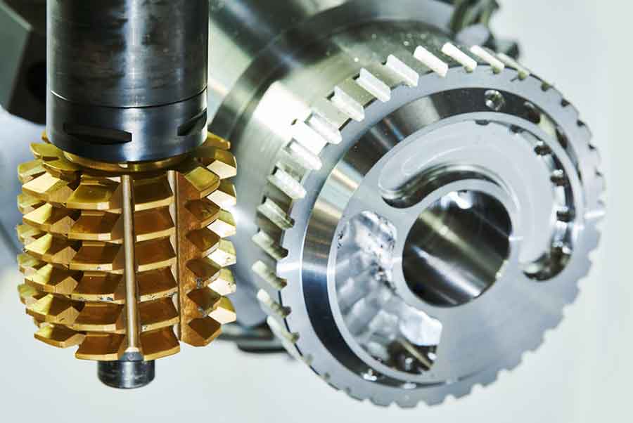
I begin from the principle that gear hobbing is not a simple copying process. The hob and the gear blank rotate in a strict relationship, while the hob also feeds along the gear axis. The generated tooth surface is the envelope of many cutting-edge positions. Therefore, any prediction of tooth surface roughness in gear hobbing must consider the relative motion, the cutting-edge geometry, the material response, and the process parameters together. I organize my work around this idea and use both theoretical and experimental evidence to support each model.
1. Kinematic and Geometric Basis of Gear Hobbing
In gear hobbing, I define the shaft angle between the hob axis and the gear axis as the difference between the gear helix angle and the hob lead angle. The center distance is the sum of the hob radius and the gear radius. These two quantities determine the initial spatial relationship between the tool and the workpiece.
$$ \Sigma = \beta – \lambda $$
$$ a = r_h + r_g $$
During gear hobbing, the hob and the gear blank must rotate according to a fixed transmission ratio. I express this ratio in the form
$$ \frac{\phi_g}{\phi_h} = \frac{Z_h}{Z_g} + \frac{\zeta}{p_g} $$
where \(Z_h\) is the number of hob starts, \(Z_g\) is the number of gear teeth, \(\phi_h\) and \(\phi_g\) are the rotation angles of the hob and gear, \(\zeta\) is the axial feed, and \(p_g\) is the gear lead. The axial feed motion in gear hobbing is essential because the hob must sweep across the full face width of the gear. I write the axial displacement as
$$ z_h = \frac{n f}{2\pi}\phi_h $$
where \(n\) is the hob rotational speed and \(f\) is the axial feed per gear revolution. If the gear hobbing operation uses radial infeed or diagonal feed, additional terms appear. I represent the radial feed function as
$$ \rho(\phi) = \rho_0 + \int v_\rho(\phi)\,d\phi $$
and the combined radial position as
$$ \rho(\phi) = \frac{D_h + D_g}{2} – d_d + \int v_\rho(\phi)\,d\phi $$
where \(D_h\) and \(D_g\) are the hob and gear outside diameters, \(d_d\) is the cutting depth, and \(v_\rho(\phi)\) is the radial feed rate. For gear hobbing, I also use homogeneous coordinate transformations to map the cutting-edge trajectory from the hob coordinate system to the gear coordinate system. The basic rotation matrices are
$$ R_x(\theta) = \begin{bmatrix} 1 & 0 & 0 & 0 \\ 0 & \cos\theta & -\sin\theta & 0 \\ 0 & \sin\theta & \cos\theta & 0 \\ 0 & 0 & 0 & 1 \end{bmatrix} $$
$$ R_y(\theta) = \begin{bmatrix} \cos\theta & 0 & \sin\theta & 0 \\ 0 & 1 & 0 & 0 \\ -\sin\theta & 0 & \cos\theta & 0 \\ 0 & 0 & 0 & 1 \end{bmatrix} $$
$$ R_z(\theta) = \begin{bmatrix} \cos\theta & -\sin\theta & 0 & 0 \\ \sin\theta & \cos\theta & 0 & 0 \\ 0 & 0 & 1 & 0 \\ 0 & 0 & 0 & 1 \end{bmatrix} $$
I model the rack profile that generates the hob worm. The rack normal section can be described by a piecewise curve. I write the general position vector as
$$ \mathbf{r}_n(u) = [x_n(u), 0, z_n(u), 1]^T $$
and the rack surface after translation along the tooth width direction as
$$ \mathbf{r}(u,v) = M_{rn} \mathbf{r}_n(u) $$
where
$$ M_{rn} = \begin{bmatrix} 1 & 0 & 0 & 0 \\ 0 & \cos\lambda & -\sin\lambda & v\cos\lambda \\ 0 & \sin\lambda & \cos\lambda & v\sin\lambda \\ 0 & 0 & 0 & 1 \end{bmatrix} $$
The hob worm surface is generated by the rack motion. I use the coordinate transformation
$$ \mathbf{r}_w(u,v,\phi_w) = M_{w,wo} M_{wo,ro} M_{ro,r} \mathbf{r}_r(u,v) $$
with the meshing condition
$$ f(u,v,\phi_w) = \left( \frac{\partial \mathbf{r}_w}{\partial u} \times \frac{\partial \mathbf{r}_w}{\partial v} \right) \cdot \frac{\partial \mathbf{r}_w}{\partial \phi_w} = 0 $$
For the gear tooth surface in gear hobbing, I extend the same idea. The generated gear surface is the envelope of the hob cutting edges under the relative motion. I write the gear surface family as
$$ \mathbf{r}_g(u,\theta,\phi_h,\zeta) = M_{g,go} M_{go,ho} M_{h,ho} \mathbf{r}_h(u,\theta) $$
The meshing equations for gear hobbing must satisfy two independent motion parameters, namely the hob rotation \(\phi_h\) and the axial feed \(\zeta\). Therefore, I require
$$ f_h(u,\theta,\phi_h,\zeta) = \left( \frac{\partial \mathbf{r}_g}{\partial u} \times \frac{\partial \mathbf{r}_g}{\partial \theta} \right) \cdot \frac{\partial \mathbf{r}_g}{\partial \phi_h} = 0 $$
$$ f_\zeta(u,\theta,\phi_h,\zeta) = \left( \frac{\partial \mathbf{r}_g}{\partial u} \times \frac{\partial \mathbf{r}_g}{\partial \theta} \right) \cdot \frac{\partial \mathbf{r}_g}{\partial \zeta} = 0 $$
This formulation gives me the basis for understanding why the tooth surface in gear hobbing contains regular tool marks, small envelopes, and local deviations. I then use a virtual gear hobbing simulation to visualize the generated surface. The simulation confirms that the tooth flank is covered by repeated cutting traces, and these traces are directly related to the process parameters.
| Hob Parameter | Value | Gear Parameter | Value |
|---|---|---|---|
| Normal module | 1.5 mm | Module | 1.5 mm |
| Normal pressure angle | 20° | Pressure angle | 20° |
| Number of starts | 1 | Number of teeth | 59 |
| Lead angle | 3°3′ | Helix angle | 0° |
| Outside diameter | 32 mm | Face width | 28 mm |
| Length | 50 mm | Material | 20CrMnTi |
| Hand | Right | Machining type | Dry gear hobbing |
2. Experimental Study of Gear Hobbing Parameters on Tooth Surface Roughness
I designed my experiments to capture the influence of gear hobbing parameters on tooth surface roughness. The main variables were hob rotational speed \(n\), axial feed speed \(v\), and radial cutting depth \(\rho\). I used a 20CrMnTi gear blank because this material is common in high-load transmission gears and has good hardenability and fatigue resistance. The chemical composition and mechanical properties are summarized below.
| Element | Mass Fraction (%) | Property | Value |
|---|---|---|---|
| C | 0.17–0.23 | Density | 7800 kg/m³ |
| Si | 0.17–0.37 | Poisson ratio | 0.25 |
| Mn | 0.80–1.10 | Elastic modulus | 207 GPa |
| S | ≤0.035 | Yield strength | 850 MPa |
| P | ≤0.035 | Tensile strength | 1147 MPa |
| Cr | 1.00–1.30 | Elongation | 10% |
| Ni | ≤0.030 | — | — |
| Cu | ≤0.030 | — | — |
| Ti | 0.04–0.10 | — | — |
I measured the tooth surface morphology with a white-light interferometer. For each gear, I selected three teeth and two regions near the pitch line on each tooth. I averaged the six measurement regions to reduce random error. The measuring area was approximately \(1736.296\,\mu m \times 1736.296\,\mu m\). I used two three-dimensional roughness parameters: the arithmetic mean height \(Sa\) and the root mean square height \(Sq\).
$$ Sa = \frac{1}{n}\sum_{i=1}^{n} |Z_i| $$
$$ Sq = \sqrt{\frac{1}{n}\sum_{i=1}^{n} Z_i^2} $$
where \(n\) is the number of measured points and \(Z_i\) is the height of point \(i\) relative to the mean plane. I prefer \(Sa\) and \(Sq\) because they describe the whole measured area more completely than a single two-dimensional profile. In gear hobbing, the tooth surface is three-dimensional and anisotropic, so three-dimensional parameters are more suitable for my prediction models.
2.1 Single-Factor Experiments in Gear Hobbing
I first performed single-factor experiments to observe the trend of tooth surface roughness when one gear hobbing parameter changes while the others remain constant. The factor levels are shown in the table below.
| Group | Hob Speed \(n\) (r/min) | Axial Feed \(v\) (mm/min) | Radial Depth \(\rho\) (mm) |
|---|---|---|---|
| 1 | 450, 600, 750, 900 | 3.5 | 1.125 |
| 2 | 900 | 2, 2.75, 3.5, 4 | 1.125 |
| 3 | 900 | 3.5 | 0.84375, 1.125, 1.6875, 3.375 |
The measured single-factor results are given below. I use these data to identify the monotonic or non-monotonic trends of gear hobbing.
| No. | \(n\) (r/min) | \(v\) (mm/min) | \(\rho\) (mm) | \(Sa\) (μm) | \(Sq\) (μm) |
|---|---|---|---|---|---|
| 1 | 450 | 3.5 | 1.125 | 0.56 | 0.74 |
| 2 | 600 | 3.5 | 1.125 | 0.51 | 0.67 |
| 3 | 750 | 3.5 | 1.125 | 0.46 | 0.58 |
| 4 | 900 | 3.5 | 1.125 | 0.25 | 0.33 |
| 5 | 900 | 2 | 1.125 | 0.19 | 0.25 |
| 6 | 900 | 2.75 | 1.125 | 0.24 | 0.31 |
| 7 | 900 | 3.5 | 1.125 | 0.22 | 0.29 |
| 8 | 900 | 4 | 1.125 | 0.73 | 0.91 |
| 9 | 900 | 3.5 | 3.375 | 0.35 | 0.44 |
| 10 | 900 | 3.5 | 1.6875 | 0.56 | 0.69 |
| 11 | 900 | 3.5 | 1.125 | 0.66 | 0.87 |
| 12 | 900 | 3.5 | 0.84375 | 0.37 | 0.48 |
For hob speed, I observe that both \(Sa\) and \(Sq\) decrease as \(n\) increases. The reason is that a higher hob speed increases the number of cutting actions per unit feed. The residual scallop height becomes smaller, and the tooth surface roughness decreases. After \(n\) exceeds 750 r/min, the thermal effect becomes stronger, the material softens locally, and the cutting marks are removed more easily. This further improves the gear hobbing surface quality.
For axial feed speed, I observe that \(Sa\) and \(Sq\) generally increase with \(v\). A higher axial feed in gear hobbing removes more material per unit time, which raises the cutting force and friction. The material undergoes incomplete plastic deformation, and micro-cracks or burrs can form on the tooth flank. Therefore, the tooth surface roughness increases. This trend indicates that I should not increase the axial feed speed too much if I want a low-roughness gear hobbing surface.
For radial cutting depth, I observe a non-monotonic trend. \(Sa\) and \(Sq\) first increase rapidly and then decrease. At small radial depths, the cutting force distribution changes, and material pile-up occurs. When the radial depth becomes larger than a critical value, the friction heat softens the material, chip evacuation improves, and the roughness decreases. In gear hobbing, the radial depth is therefore not simply a “larger is worse” variable; it interacts strongly with thermal and chip removal effects.
2.2 Response Surface Experiments for Gear Hobbing
To capture interactions among gear hobbing parameters, I used a Box-Behnken design. The factors and levels are listed below.
| Level | \(n\) (r/min) | \(v\) (mm/min) | \(\rho\) (mm) |
|---|---|---|---|
| -1 | 450 | 2 | 0.843 |
| 0 | 600 | 2.75 | 1.125 |
| 1 | 750 | 3.5 | 1.687 |
The response surface design and measured tooth surface roughness values are shown in the following table. Each run represents a gear hobbing experiment with a specific parameter combination.
| No. | \(n\) (r/min) | \(v\) (mm/min) | \(\rho\) (mm) | \(Sa\) (μm) | \(Sq\) (μm) |
|---|---|---|---|---|---|
| 1 | 600 | 2.75 | 1.125 | 0.46 | 0.65 |
| 2 | 750 | 2 | 1.125 | 0.58 | 0.74 |
| 3 | 600 | 3.5 | 0.84375 | 0.31 | 0.58 |
| 4 | 600 | 2.75 | 1.125 | 0.40 | 0.63 |
| 5 | 750 | 3.5 | 1.125 | 0.30 | 0.59 |
| 6 | 600 | 2 | 1.6875 | 0.42 | 0.65 |
| 7 | 750 | 2.75 | 0.84375 | 0.28 | 0.46 |
| 8 | 750 | 2.75 | 1.6875 | 0.43 | 0.64 |
| 9 | 450 | 3.5 | 1.125 | 0.59 | 0.77 |
| 10 | 600 | 2.75 | 1.125 | 0.45 | 0.65 |
| 11 | 600 | 2 | 0.84375 | 0.42 | 0.68 |
| 12 | 600 | 3.5 | 1.6875 | 0.42 | 0.56 |
| 13 | 450 | 2.75 | 1.6875 | 0.47 | 0.55 |
| 14 | 600 | 2.75 | 1.125 | 0.45 | 0.68 |
| 15 | 450 | 2.75 | 0.84375 | 0.65 | 0.70 |
| 16 | 600 | 2.75 | 1.125 | 0.42 | 0.66 |
| 17 | 450 | 2 | 1.125 | 0.56 | 0.73 |
Using the coded variables \(A\), \(B\), and \(C\) for hob speed, axial feed speed, and radial depth, I obtained the response surface model for \(Sa\):
$$ Sa = 0.4455 – 0.0729A – 0.0391B + 0.0095C – 0.0775AB + 0.0726AC + 0.0327BC + 0.0688A^2 – 0.0027B^2 – 0.0567C^2 $$
The response surface model for \(Sq\) is
$$ Sq = 0.6628 – 0.0268A – 0.0376B – 0.0025C – 0.0475AB + 0.0789AC – 0.0008BC + 0.0117A^2 + 0.0417B^2 – 0.0871C^2 $$
I evaluated the significance of these gear hobbing models by analysis of variance. The results for \(Sa\) are given below.
| Source | Sum of Squares | DF | Mean Square | F Value | P Value | Significance |
|---|---|---|---|---|---|---|
| Model | 0.1532 | 9 | 0.0170 | 8.78 | 0.0046 | Significant |
| A | 0.0404 | 1 | 0.0404 | 20.84 | 0.0026 | — |
| B | 0.0116 | 1 | 0.0116 | 5.98 | 0.0444 | — |
| C | 0.0007 | 1 | 0.0007 | 0.3726 | 0.5609 | — |
| AB | 0.0240 | 1 | 0.0240 | 12.40 | 0.0097 | — |
| AC | 0.0223 | 1 | 0.0223 | 11.49 | 0.0116 | — |
| BC | 0.0045 | 1 | 0.0045 | 2.33 | 0.1709 | — |
| \(A^2\) | 0.0199 | 1 | 0.0199 | 10.27 | 0.0150 | — |
| \(B^2\) | 0.0000 | 1 | 0.0000 | 0.0164 | 0.9016 | — |
| \(C^2\) | 0.0101 | 1 | 0.0101 | 5.22 | 0.0563 | — |
| Residual | 0.0136 | 7 | 0.0019 | — | — | — |
| Lack of Fit | 0.0110 | 3 | 0.0037 | 5.84 | 0.0606 | Not significant |
| Pure Error | 0.0025 | 4 | 0.0006 | — | — | — |
| Total | 0.1667 | 16 | — | — | — | — |
For \(Sa\), the model is significant with \(F=8.78\) and \(P=0.0046\). The lack-of-fit P value is 0.0606, which means the lack of fit is not significant. The coefficient of determination is \(R^2=0.9187\), and the adjusted value is \(R^2_{Adj}=0.8141\). The order of influence on \(Sa\) is \(A > B > C\), so hob speed is the strongest factor in this gear hobbing response model.
For \(Sq\), the analysis of variance is shown below.
| Source | Sum of Squares | DF | Mean Square | F Value | P Value | Significance |
|---|---|---|---|---|---|---|
| Model | 0.0916 | 9 | 0.0102 | 18.26 | 0.0005 | Significant |
| A | 0.0055 | 1 | 0.0055 | 9.82 | 0.0165 | — |
| B | 0.0108 | 1 | 0.0108 | 19.31 | 0.0032 | — |
| C | 0.0000 | 1 | 0.0000 | 0.0897 | 0.7732 | — |
| AB | 0.0090 | 1 | 0.0090 | 16.19 | 0.0050 | — |
| AC | 0.0263 | 1 | 0.0263 | 47.21 | 0.0002 | — |
| BC | 2.632E-06 | 1 | 2.632E-06 | 0.0047 | 0.9471 | — |
| \(A^2\) | 0.0006 | 1 | 0.0006 | 1.04 | 0.3411 | — |
| \(B^2\) | 0.0073 | 1 | 0.0073 | 13.17 | 0.0084 | — |
| \(C^2\) | 0.0238 | 1 | 0.0238 | 42.77 | 0.0003 | — |
| Residual | 0.0039 | 7 | 0.0006 | — | — | — |
| Lack of Fit | 0.0026 | 3 | 0.0009 | 2.61 | 0.1886 | Not significant |
| Pure Error | 0.0013 | 4 | 0.0003 | — | — | — |
| Total | 0.0955 | 16 | — | — | — | — |
For \(Sq\), the model is significant with \(F=18.26\) and \(P=0.0005\). The lack-of-fit P value is 0.1886, so the lack of fit is not significant. The coefficient of determination is \(R^2=0.9591\), and the adjusted value is \(R^2_{Adj}=0.9066\). The order of influence on \(Sq\) is \(B > A > C\), so axial feed speed is the strongest factor for \(Sq\) in my gear hobbing experiments.
I also analyzed the residuals to check model adequacy. The residual is defined as
$$ e_i = y_i – \hat{y}_i $$
and the externally standardized residual is
$$ t_i = \frac{e_i}{\sigma \sqrt{1-h_{ii}}} $$
where the leverage values come from the hat matrix
$$ H = X(X^T X)^{-1} X^T $$
I plotted the residuals against normal probability and predicted values. The residuals lie approximately along the reference line and are randomly scattered within \(\pm 2\). This behavior supports the normality assumption and confirms that my response surface models for gear hobbing are reliable within the tested range.
3. Machine Learning Prediction Models for Gear Hobbing Roughness
The response surface model is useful, but it is still a quadratic polynomial. Gear hobbing is strongly nonlinear because the cutting edges, contact conditions, and thermal effects interact. Therefore, I built two machine learning models: a back-propagation neural network optimized by a sparrow search algorithm, and a support vector machine optimized by particle swarm optimization. I used the response surface experimental data to train and test both models. The input variables were hob speed, axial feed speed, and radial cutting depth. The outputs were \(Sa\) and \(Sq\).
3.1 BP Neural Network and Sparrow Search Optimization
A classical BP neural network contains an input layer, one or more hidden layers, and an output layer. For each neuron, I write the output as
$$ y = f\left(\sum_{i=1}^{m} w_i x_i + b\right) $$
where \(w_i\) are weights, \(b\) is the bias, and \(f\) is the activation function. The network updates weights and biases by back-propagating the error. However, a BP network can become trapped in a local minimum. To avoid this, I used the sparrow search algorithm to optimize the initial weights and biases.
In the sparrow search algorithm, the population is divided into producers and scroungers. The producer position update is
$$ X_{i,j}^{t+1} = \begin{cases} X_{i,j}^{t} \exp\left(-\frac{i}{\alpha N}\right), & R_2 < ST \\ X_{i,j}^{t} + QL, & R_2 \ge ST \end{cases} $$
The scrounger position update is
$$ X_{i,j}^{t+1} = \begin{cases} Q \exp\left(\frac{X_{\text{worst}} – X_{i,j}^{t}}{i^2}\right), & i > n/2 \\ X_{P}^{t+1} + |X_{i,j}^{t} – X_{P}^{t+1}| A^+ L, & \text{otherwise} \end{cases} $$
The anti-predation position update is
$$ X_{i,j}^{t+1} = \begin{cases} X_{\text{best}}^{t} + \beta |X_{i,j}^{t} – X_{\text{best}}^{t}|, & f_i > f_{\text{best}} \\ X_{i,j}^{t} + K \left( \frac{|X_{i,j}^{t} – X_{\text{worst}}^{t}|}{(f_i – f_{\text{worst}}) + \epsilon} \right), & f_i = f_{\text{best}} \end{cases} $$
I used the mean squared error of the training and test sets as the fitness function:
$$ f = \frac{R_{Mse1} + R_{Mse2}}{2} $$
I tested different hidden-layer node numbers. The average root mean square errors are shown below.
| Hidden Nodes | Run 1 | Run 2 | Run 3 | Average RMSE | Rank |
|---|---|---|---|---|---|
| 3 | 0.0494 | 0.0992 | 0.0707 | 0.0731 | 3 |
| 4 | 0.0390 | 0.0432 | 0.0387 | 0.0403 | 1 |
| 5 | 0.0655 | 0.1349 | 0.0616 | 0.0873 | 5 |
| 6 | 0.0743 | 0.1026 | 0.1271 | 0.1013 | 7 |
| 7 | 0.0665 | 0.1254 | 0.0595 | 0.0838 | 4 |
| 8 | 0.0607 | 0.0721 | 0.0681 | 0.0670 | 2 |
| 9 | 0.1020 | 0.1065 | 0.0981 | 0.1022 | 8 |
| 10 | 0.1389 | 0.0594 | 0.0706 | 0.0896 | 6 |
According to my tests, four hidden nodes gave the lowest average RMSE. I also selected a population size of 40 because it gave the fastest convergence and the smallest fitness value. The SSA-BP model reached a fitness of about 0.037 at the sixth generation. The final SSA-BP structure was 3-4-2. The training iteration number was 800, the maximum SSA iteration was 15, the learning rate was 0.01, and the minimum training error target was \(1\times 10^{-5}\).
After training, the SSA-BP model achieved a coefficient of determination of \(R^2=0.9307\) for \(Sa\) and \(R^2=0.9696\) for \(Sq\). These values show that the SSA-BP model can approximate the gear hobbing roughness response reasonably well.
3.2 Support Vector Machine and Particle Swarm Optimization
A support vector machine seeks an optimal separating hyperplane. For a nonlinear problem, I map the input data into a higher-dimensional space. The primal optimization problem is
$$ \min_{w,b} \frac{1}{2}\|w\|^2 $$
$$ \text{subject to } y_i(w^T x_i + b) \ge 1, \quad i=1,\dots,l $$
The dual problem is
$$ \max_{\alpha} \sum_{i=1}^{l} \alpha_i – \frac{1}{2}\sum_{i=1}^{l}\sum_{j=1}^{l} \alpha_i \alpha_j y_i y_j x_i^T x_j $$
$$ \text{subject to } \sum_{i=1}^{l} \alpha_i y_i = 0, \quad \alpha_i \ge 0 $$
I use a Gaussian radial basis kernel because it maps nonlinear gear hobbing data into a high-dimensional feature space and has good convergence behavior:
$$ K(x_i,x_j) = \exp\left(-\frac{\|x_i – x_j\|^2}{2\sigma^2}\right) $$
Particle swarm optimization is used to select the penalty parameter and kernel parameter. The velocity and position updates are
$$ v_{id}^{t+1} = \omega v_{id}^{t} + c_1 r_1(p_{id} – x_{id}^{t}) + c_2 r_2(p_{gd} – x_{id}^{t}) $$
$$ x_{id}^{t+1} = x_{id}^{t} + v_{id}^{t+1} $$
I set the maximum particle number to 20, the maximum evolution number to 100, the learning factors to \(c_1=1.5\) and \(c_2=1.7\), the penalty parameter range to \([0.1,100]\), and the kernel parameter range to \([0.1,100]\). I also tested the hidden node number for the PSO-SVM model.
| Hidden Nodes | Run 1 | Run 2 | Run 3 | Average RMSE | Rank |
|---|---|---|---|---|---|
| 3 | 0.0377 | 0.1350 | 0.0410 | 0.0712 | 3 |
| 4 | 0.0644 | 0.0705 | 0.0610 | 0.0653 | 1 |
| 5 | 0.0742 | 0.1213 | 0.0828 | 0.0928 | 4 |
| 6 | 0.0584 | 0.0861 | 0.0601 | 0.0682 | 2 |
| 7 | 0.1012 | 0.1696 | 0.1341 | 0.1350 | 5 |
| 8 | 0.1362 | 0.2657 | 0.3624 | 0.2548 | 8 |
| 9 | 0.1805 | 0.1780 | 0.1789 | 0.1691 | 6 |
| 10 | 0.4713 | 0.0553 | 0.1013 | 0.2093 | 7 |
The best hidden node number for the PSO-SVM model was also four. The final PSO-SVM model reached \(R^2=0.9562\) for \(Sa\) and \(R^2=0.9882\) for \(Sq\). These values are higher than those of the SSA-BP model, which suggests that the PSO-SVM model captures the nonlinear relationship in gear hobbing more accurately.
3.3 Comparison of Prediction Models
I compared the response surface model, the SSA-BP model, and the PSO-SVM model using mean absolute error, mean squared error, mean absolute percentage error, and the coefficient of determination. The formulas are
$$ MAE = \frac{1}{m}\sum_{i=1}^{m} |y_i – \hat{y}_i| $$
$$ MSE = \frac{1}{m}\sum_{i=1}^{m} (y_i – \hat{y}_i)^2 $$
$$ MAPE = \frac{1}{m}\sum_{i=1}^{m} \left| \frac{y_i – \hat{y}_i}{y_i} \right| $$
The comparison is summarized below.
| Output | Model | MAE | MSE | MAPE (%) | \(R^2\) |
|---|---|---|---|---|---|
| \(Sa\) | RSM | 0.02704 | 0.00152 | 0.03547 | 0.9187 |
| SSA-BP | 0.02132 | 0.00056 | 0.05224 | 0.9307 | |
| PSO-SVM | 0.01828 | 0.00045 | 0.04234 | 0.9562 | |
| \(Sq\) | RSM | 0.00871 | 0.00015 | 0.01297 | 0.9591 |
| SSA-BP | 0.00542 | 0.00006 | 0.00801 | 0.9696 | |
| PSO-SVM | 0.00377 | 0.00001 | 0.00583 | 0.9882 |
Both machine learning models outperform the response surface model in terms of \(R^2\) and error metrics. Among them, the PSO-SVM model has the lowest MAE, MSE, and MAPE values for both \(Sa\) and \(Sq\). Therefore, I select the PSO-SVM model as the fitness function for my multi-objective optimization of gear hobbing parameters.
4. Multi-Objective Optimization of Gear Hobbing Parameters
After obtaining a reliable prediction model, I formulate the gear hobbing parameter optimization problem. I treat hob speed \(n\), axial feed speed \(v\), and radial cutting depth \(\rho\) as decision variables. I aim to minimize tooth surface roughness and transient cutting force. The objective functions are
$$ F_1 = \text{PSO-SVM}_{Sa}(n,v,\rho) $$
$$ F_2 = \text{PSO-SVM}_{Sq}(n,v,\rho) $$
$$ F_3 = F_c = K n^{0.8} v^{0.6} \rho^{1.2} HB^{-1} $$
where \(K\) is a tool-material interaction coefficient and \(HB\) is the workpiece hardness. I set the constraints according to my experimental range and practical gear hobbing conditions:
$$ 450 \le n \le 750 $$
$$ 2 \le v \le 3.5 $$
$$ 0.84375 \le \rho \le 1.6875 $$
The multi-objective optimization problem can be written as
$$ \min_{X} F(X) = [F_1(X), F_2(X), F_3(X)]^T $$
$$ X = [n, v, \rho]^T \in \mathbb{R}^3 $$
I solve this problem with the non-dominated sorting genetic algorithm II. The main steps are:
1. Initialize a random parent population within the gear hobbing parameter bounds.
2. Evaluate all objective functions by using the PSO-SVM prediction model and the transient cutting force equation.
3. Perform fast non-dominated sorting and crowding-distance calculation.
4. Apply selection, crossover, and mutation to generate an offspring population.
5. Combine parent and offspring populations and apply elitist retention.
6. Repeat until the maximum generation number is reached.
I use the following formulas for non-dominated sorting and crowding distance. A solution \(X_1\) dominates \(X_2\) if
$$ \forall i \in \{1,\dots,m\}, \quad f_i(X_1) \le f_i(X_2) $$
and
$$ \exists j \in \{1,\dots,m\}, \quad f_j(X_1) < f_j(X_2) $$
The crowding distance for a solution \(i\) is
$$ CD_i = \sum_{k=1}^{m} \frac{f_k(i+1) – f_k(i-1)}{f_k^{\max} – f_k^{\min}} $$
A larger crowding distance means that the solution lies in a less crowded region of the Pareto front, so I prefer it when the non-domination ranks are equal.
4.1 Two-Objective Optimization Results
First, I optimized \(Sa\) and transient cutting force. The Pareto front shows a trade-off: when \(Sa\) decreases, the transient cutting force tends to increase. I selected a balanced region where \(F_c\) is between 2.0 and 3.1 and \(Sa\) is between 0.30 and 0.37. Some representative parameter combinations are listed below.
| No. | \(n\) (r/min) | \(v\) (mm/min) | \(\rho\) (mm) | \(Sa\) (μm) | \(F_c\) (kN) |
|---|---|---|---|---|---|
| 1 | 701.4 | 2.31 | 1.41 | 0.340 | 3.19 |
| 2 | 452.6 | 2.11 | 0.79 | 0.316 | 2.14 |
| 3 | 589.4 | 3.07 | 1.167 | 0.308 | 2.94 |
| 4 | 611.9 | 2.97 | 1.066 | 0.364 | 3.09 |
| 5 | 651.3 | 2.46 | 0.805 | 0.365 | 2.94 |
| 6 | 705.7 | 3.11 | 0.976 | 0.302 | 2.42 |
| 7 | 483.5 | 2.03 | 1.725 | 0.365 | 2.81 |
| 8 | 450.0 | 1.89 | 1.08 | 0.319 | 2.73 |
I also optimized \(Sq\) and transient cutting force. In this case, the balanced region has \(F_c\) between 2.7 and 3.7 and \(Sq\) between 0.55 and 0.60. Representative solutions are shown below.
| No. | \(n\) (r/min) | \(v\) (mm/min) | \(\rho\) (mm) | \(Sq\) (μm) | \(F_c\) (kN) |
|---|---|---|---|---|---|
| 1 | 695.9 | 1.95 | 0.95 | 0.607 | 2.89 |
| 2 | 503.6 | 3.427 | 0.811 | 0.561 | 3.60 |
| 3 | 614.0 | 3.292 | 0.891 | 0.573 | 3.36 |
| 4 | 466.2 | 3.35 | 0.797 | 0.581 | 3.08 |
| 5 | 685.0 | 1.93 | 0.949 | 0.578 | 3.31 |
| 6 | 779.3 | 2.21 | 1.77 | 0.566 | 3.43 |
4.2 Three-Objective Optimization Results
I then solved the three-objective problem including \(Sa\), \(Sq\), and transient cutting force. The NSGA-II algorithm returned 51 Pareto solutions with a population size of 100 and 100 generations. Some representative solutions are given below.
| No. | \(n\) (r/min) | \(v\) (mm/min) | \(\rho\) (mm) | \(Sa\) (μm) | \(Sq\) (μm) | \(F_c\) (kN) |
|---|---|---|---|---|---|---|
| 1 | 420.0 | 1.59 | 0.710 | 0.605 | 0.764 | 4.860 |
| 2 | 420.0 | 1.85 | 0.759 | 0.268 | 0.506 | 5.160 |
| 3 | 725.0 | 3.48 | 1.172 | 0.466 | 0.688 | 1.577 |
| 4 | 560.0 | 2.15 | 0.778 | 0.288 | 0.577 | 3.100 |
| 5 | 451.4 | 1.85 | 0.764 | 0.435 | 0.680 | 1.635 |
| 6 | 628.4 | 2.21 | 0.766 | 0.387 | 0.631 | 2.190 |
| 7 | 695.8 | 2.35 | 0.929 | 0.425 | 0.677 | 1.682 |
| 8 | 489.8 | 1.85 | 0.760 | 0.316 | 0.612 | 2.546 |
| 9 | 495.5 | 1.90 | 0.760 | 0.383 | 0.628 | 2.290 |
Because the three objectives have different importance in gear hobbing, I use a combination weighting method. The subjective weights are 0.35 for \(Sa\), 0.35 for \(Sq\), and 0.30 for transient cutting force. I also calculate objective weights by the entropy method. The normalization for a negative indicator is
$$ X_{ij} = \frac{s_{\max} – s_{ij}}{s_{\max} – s_{\min}} $$
The entropy of indicator \(j\) is
$$ e_j = -k \sum_{i=1}^{n} p_{ij} \ln p_{ij} $$
where \(k = 1/\ln n\) and \(p_{ij}\) is the proportion of the \(i\)-th value in the \(j\)-th indicator. The redundancy is
$$ d_j = 1 – e_j $$
and the objective weight is
$$ w_j = \frac{d_j}{\sum_{j=1}^{m} d_j} $$
The entropy weights I obtained are shown below.
| Objective | Entropy \(e\) | Redundancy \(d\) | Weight (%) |
|---|---|---|---|
| \(Sa\) | 0.950 | 0.050 | 17.182 |
| \(Sq\) | 0.979 | 0.021 | 7.139 |
| \(F_c\) | 0.969 | 0.031 | 10.659 |
I combine the subjective and objective weights by
$$ Q_j = \frac{\alpha_j \beta_j}{\sum_{j=1}^{m} \alpha_j \beta_j} $$
The final combined weights are listed below.
| Objective | Subjective Weight | Entropy Weight | Combined Weight |
|---|---|---|---|
| \(Sa\) | 0.350 | 0.172 | 0.421 |
| \(Sq\) | 0.350 | 0.071 | 0.277 |
| \(F_c\) | 0.300 | 0.107 | 0.303 |
I rank all Pareto solutions by the combined score. The top ten solutions are presented below.
| Rank | \(n\) (r/min) | \(v\) (mm/min) | \(\rho\) (mm) | \(Sa\) (μm) | \(Sq\) (μm) | \(F_c\) (kN) | Score |
|---|---|---|---|---|---|---|---|
| 1 | 705.5 | 3.15 | 1.738 | 0.390 | 0.658 | 2.96 | 0.7449 |
| 2 | 763.0 | 3.54 | 1.082 | 0.295 | 0.590 | 2.90 | 0.7158 |
| 3 | 736.3 | 2.75 | 1.372 | 0.292 | 0.613 | 2.96 | 0.7025 |
| 4 | 768.8 | 2.28 | 1.730 | 0.538 | 0.677 | 1.75 | 0.6523 |
| 5 | 714.8 | 3.35 | 1.359 | 0.485 | 0.618 | 2.69 | 0.6282 |
| 6 | 700.4 | 3.24 | 1.374 | 0.447 | 0.657 | 2.81 | 0.6183 |
| 7 | 656.8 | 3.00 | 1.620 | 0.525 | 0.650 | 2.17 | 0.6148 |
| 8 | 705.7 | 3.10 | 0.976 | 0.302 | 0.617 | 2.42 | 0.6139 |
| 9 | 483.1 | 3.43 | 1.728 | 0.474 | 0.648 | 2.00 | 0.6069 |
| 10 | 557.7 | 3.15 | 1.377 | 0.329 | 0.627 | 2.63 | 0.6066 |
I select the first ranked solution as the recommended three-objective gear hobbing parameter set. It gives \(n=705.5\) r/min, \(v=3.15\) mm/min, and \(\rho=1.738\) mm, with \(Sa=0.390\,\mu m\), \(Sq=0.658\,\mu m\), and \(F_c=2.96\,kN\). This combination balances tooth surface roughness and transient cutting force in my model.
4.3 Comparison with Empirical Gear Hobbing Parameters
To verify the optimization effect, I compared my optimized solutions with an empirical gear hobbing parameter set. The empirical set was \(n=600\) r/min, \(v=3.0\) mm/min, and \(\rho=1.25\) mm. The measured or estimated responses were \(Sa=0.403\,\mu m\), \(Sq=0.663\,\mu m\), and \(F_c=3.26\,kN\). The comparison is shown below.
| Case | \(n\) (r/min) | \(v\) (mm/min) | \(\rho\) (mm) | \(Sa\) (μm) | \(Sq\) (μm) | \(F_c\) (kN) |
|---|---|---|---|---|---|---|
| Optimized \(Sa\) + \(F_c\) | 705.7 | 3.11 | 0.976 | 0.302 | — | 2.42 |
| Optimized \(Sq\) + \(F_c\) | 614.0 | 3.292 | 0.891 | — | 0.573 | 3.36 |
| Optimized \(Sa\) + \(Sq\) + \(F_c\) | 705.5 | 3.15 | 1.738 | 0.390 | 0.658 | 2.96 |
| Empirical | 600.0 | 3.00 | 1.250 | 0.403 | 0.663 | 3.26 |
The improvement relative to the empirical values is summarized below.
| Comparison | \(Sa\) Reduction (%) | \(Sq\) Reduction (%) | \(F_c\) Reduction (%) |
|---|---|---|---|
| Optimized \(Sa\) + \(F_c\) vs empirical | 33.4 | — | 34.7 |
| Optimized \(Sq\) + \(F_c\) vs empirical | — | 15.7 | 3.3 |
| Three-objective vs empirical | 3.3 | 0.76 | 10.1 |
I find that the two-objective solutions produce large reductions in one or two selected objectives, while the three-objective solution provides a more balanced improvement. In gear hobbing, this balance is important because a very low roughness value may require a cutting force that is too high for the tool or machine. My combined weighting method therefore helps me select a practical parameter set rather than a purely mathematical optimum.
5. Discussion
My study shows that gear hobbing tooth surface roughness is controlled by several interacting mechanisms. The kinematic envelope determines the basic cutting trace pattern. The hob speed changes the number of cutting actions per unit feed and the thermal conditions. The axial feed speed changes the material removal rate and the cutting force. The radial cutting depth changes the contact area, chip evacuation, and thermal softening. These effects explain why a single-factor experiment is not enough for gear hobbing optimization. The response surface experiments reveal significant interactions, especially between hob speed and axial feed speed for \(Sa\), and between hob speed and radial depth for \(Sq\).
The machine learning models improve the prediction accuracy because they do not assume a fixed polynomial form. The SSA-BP model uses a global search to optimize the initial weights and biases, which reduces the chance of local minima. The PSO-SVM model uses a kernel function and optimized hyperparameters, which gives it strong generalization ability for small experimental data sets. In my comparison, PSO-SVM gives the best \(R^2\) and the lowest error metrics for both \(Sa\) and \(Sq\). This is why I use it as the fitness function in my multi-objective gear hobbing optimization.
The NSGA-II algorithm provides a set of Pareto solutions rather than a single solution. This is valuable for gear hobbing because different production scenarios may require different compromises. For rough gear hobbing, a higher material removal rate may be acceptable, so a slightly higher roughness can be traded for lower cost. For semi-finish gear hobbing, lower roughness and moderate cutting force may be preferred. The combined weighting method allows me to rank solutions according to both subjective engineering priorities and objective data dispersion. The selected solution reduces \(Sa\), \(Sq\), and transient cutting force relative to the empirical parameter set.
6. Conclusions
I draw the following conclusions from my gear hobbing study.
1. The tooth surface in gear hobbing is generated by the envelope of hob cutting edges under coupled rotation and feed motion. The kinematic and geometric model explains the formation of regular cutting traces and provides the basis for roughness prediction.
2. Single-factor gear hobbing experiments show that \(Sa\) and \(Sq\) decrease with increasing hob speed, increase with increasing axial feed speed, and first increase and then decrease with increasing radial cutting depth.
3. Response surface models for \(Sa\) and \(Sq\) are significant within the tested gear hobbing range. For \(Sa\), the influence order is hob speed, axial feed speed, and radial depth. For \(Sq\), the influence order is axial feed speed, hob speed, and radial depth. Residual analysis confirms that the models are adequate.
4. The SSA-BP and PSO-SVM machine learning models both predict gear hobbing tooth surface roughness more accurately than the response surface model. The PSO-SVM model performs best, with \(R^2=0.9562\) for \(Sa\) and \(R^2=0.9882\) for \(Sq\).
5. The multi-objective optimization based on the PSO-SVM model and NSGA-II produces Pareto fronts for \(Sa\), \(Sq\), and transient cutting force. After combined weighting, the recommended three-objective gear hobbing parameter set is \(n=705.5\) r/min, \(v=3.15\) mm/min, and \(\rho=1.738\) mm. This set reduces roughness and cutting force relative to the empirical parameter set.
6. My results show that combining physical modeling, response surface experiments, machine learning, and multi-objective optimization is an effective way to control gear hobbing tooth surface quality. The approach can be extended to other gear hobbing conditions, materials, and tool geometries when sufficient experimental data are available.
| Stage | Method | Main Output | Key Finding |
|---|---|---|---|
| Kinematic analysis | Envelope theory | Tooth surface formation model | Gear hobbing traces come from cutting-edge envelopes |
| Single-factor test | One-variable experiments | Roughness trends | Speed reduces roughness; feed increases roughness |
| Response surface | Box-Behnken design | Quadratic models for \(Sa\) and \(Sq\) | Interactions are significant |
| Machine learning | SSA-BP and PSO-SVM | Nonlinear prediction models | PSO-SVM has the best accuracy |
| Optimization | NSGA-II and combined weighting | Pareto parameter sets | Balanced gear hobbing parameters improve quality and force |
In future work, I would extend the gear hobbing model to include tool wear, residual stress, machining energy, and production time. I would also test the optimized parameter sets on different gear materials and module sizes. These extensions would make the gear hobbing prediction and optimization framework more general and more useful for industrial gear manufacturing.