
Asymmetric involute gears offer larger load capacity, smaller volume, lower weight, and longer service life than conventional symmetric gears. Because the working flank and non-working flank use different pressure angles, the gear pair can improve bending strength, contact strength, vibration behavior, and lubrication performance. These advantages make asymmetric gears attractive for high-speed, heavy-duty, and high-power transmission systems in aerospace, marine, and industrial machinery. However, the manufacturing accuracy of asymmetric gears directly controls their transmission performance. Gear cutting is therefore a central technology for transferring asymmetric gear design into reliable engineering applications.
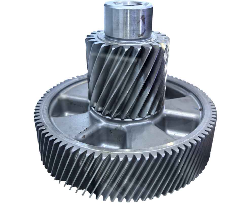
Among the available gear cutting methods, milling, hobbing, shaping, grinding, and shaving are commonly used. Hobbing is often applied for rough gear cutting, while grinding and shaving are used for finishing. Gear shaping is a generative gear cutting process that uses a pinion-type cutter. It can accurately generate external gears, internal gears, multi-connected gears, and gears with shoulders. For asymmetric gears, gear shaping has important advantages because the cutter profile can be designed according to the asymmetric involute geometry, and the generating motion can reproduce the required working and non-working flanks. In this work, I studied asymmetric involute gear modeling, gear shaping cutter design, cutter angle optimization, numerical control gear cutting simulation, and machining error analysis.
Asymmetric Involute Gear Geometry
The involute curve is formed by rolling a straight line on a base circle. For any point K on the involute, the radius, pressure angle, and involute angle satisfy the following relations. The base radius is denoted by rb, the radius at point K is rK, and the pressure angle at point K is alphaK.
$$r_K = \frac{r_b}{\cos \alpha_K}$$
$$\theta_K = \tan \alpha_K – \alpha_K = inv\,\alpha_K$$
Using the unwinding angle phiK as a parameter, the involute can be written in Cartesian coordinates as follows.
$$x_K = r_b(\cos \phi_K + \phi_K \sin \phi_K)$$
$$y_K = r_b(\sin \phi_K – \phi_K \cos \phi_K)$$
For an asymmetric spur gear, the two flanks are generated from different base circles and different pressure angles. I defined the working-side pressure angle as alphad and the non-working-side pressure angle as alphac. The working-side tooth profile for a point M can be expressed as a coordinate transformation involving the tooth thickness, involute function, and pressure angle. In compact form, the working-side profile is given by the following matrix relation.
$$\begin{bmatrix} x_M \\ y_M \end{bmatrix} =
\begin{bmatrix}
\sin\left(\frac{\pi}{2z} + inv\alpha_d – inv\alpha_{Md}\right) & \cos\left(\frac{\pi}{2z} + inv\alpha_d – inv\alpha_{Md}\right) \\
\cos\left(\frac{\pi}{2z} + inv\alpha_d – inv\alpha_{Md}\right) & -\sin\left(\frac{\pi}{2z} + inv\alpha_d – inv\alpha_{Md}\right)
\end{bmatrix}
\begin{bmatrix}
\frac{mz}{2}\cos\alpha_{Md} \\
\frac{mz}{2}\cos\alpha_{Md}
\end{bmatrix}$$
The non-working-side profile for a point N is similarly written as follows.
$$\begin{bmatrix} x_N \\ y_N \end{bmatrix} =
\begin{bmatrix}
\sin\left(\frac{\pi}{2z} + inv\alpha_c – inv\alpha_{Nc}\right) & \cos\left(\frac{\pi}{2z} + inv\alpha_c – inv\alpha_{Nc}\right) \\
\cos\left(\frac{\pi}{2z} + inv\alpha_c – inv\alpha_{Nc}\right) & -\sin\left(\frac{\pi}{2z} + inv\alpha_c – inv\alpha_{Nc}\right)
\end{bmatrix}
\begin{bmatrix}
\frac{mz}{2}\cos\alpha_{Nc} \\
\frac{mz}{2}\cos\alpha_{Nc}
\end{bmatrix}$$
For an asymmetric helical gear, the end-face involute is extended along a helix. If a point on the end face has coordinates x and y, and the helical parameter is mu, the spatial coordinates of the helical surface are obtained by rotating the end-face profile and translating it along the gear axis.
$$X = x\cos\mu – y\sin\mu$$
$$Y = x\sin\mu + y\cos\mu$$
$$Z = z + \frac{h\mu}{2\pi}$$
The lead h and the helix angle beta are related by the local radius r.
$$\beta = \arctan\left(\frac{2\pi r}{h}\right)$$
Substituting the working-side and non-working-side involute equations into the helical transformation gives the asymmetric helical gear surfaces. For the working side, the surface can be written as follows.
$$X = r_{bd}\left[\sin\left(\frac{\pi}{2z}+inv\alpha_d-inv\alpha_k\right)\cos\mu –
\cos\left(\frac{\pi}{2z}+inv\alpha_d-inv\alpha_k\right)\sin\mu\right]$$
$$Y = r_{bd}\left[\sin\left(\frac{\pi}{2z}+inv\alpha_d-inv\alpha_k\right)\sin\mu +
\cos\left(\frac{\pi}{2z}+inv\alpha_d-inv\alpha_k\right)\cos\mu\right]$$
$$Z = \frac{h\mu}{2\pi}$$
For the non-working side, the corresponding surface is expressed with alphac and the non-working involute function. These equations provide the mathematical basis for asymmetric gear solid modeling and for subsequent gear cutting tool design.
Three-Dimensional Modeling of Asymmetric Gears
I used the derived involute and helical equations to build asymmetric spur and helical gear models. The basic parameters for the asymmetric spur gear are listed in the table below. The working-side pressure angle is larger than the non-working-side pressure angle so that the working flank can carry higher contact and bending loads without making the tooth tip too sharp.
| Parameter | Value |
|---|---|
| Number of teeth z | 30 |
| Working-side pressure angle alphad | 36 degrees |
| Non-working-side pressure angle alphac | 20 degrees |
| Module m | 2 mm |
| Face width B | 20 mm |
| Addendum coefficient ha | 1 |
| Bottom clearance coefficient ck | 0.5 |
| Profile shift coefficient x | 0 |
| Shaft hole diameter | 18.5 mm |
The asymmetric helical gear used the same basic tooth parameters but included a helix angle. The helical parameters are given below.
| Parameter | Value |
|---|---|
| Number of teeth z | 30 |
| Working-side pressure angle alphad | 36 degrees |
| Non-working-side pressure angle alphac | 20 degrees |
| Module m | 2 mm |
| Helix angle beta | 20 degrees |
| Face width B | 20 mm |
| Profile shift coefficient x | 0 |
| Shaft hole diameter | 18.5 mm |
The modeling process began with mathematical expressions for the involute and root transition curves. I imported the expressions into a CAD environment, generated the working-side and non-working-side involutes, and trimmed them with the base circle, root circle, pitch circle, and addendum circle. A single asymmetric tooth profile was then extruded and patterned around the gear axis. For the helical gear, the end-face profile was swept along a helical guide curve. The resulting solid models were used for gear cutting simulation and tool design.
Gear Shaping Cutter Design
Gear shaping is a generative gear cutting process. The cutter and the workpiece rotate relative to each other like a meshing gear pair. At the same time, the cutter reciprocates along the workpiece axis to remove material. Radial feed is applied to reach the full tooth depth, and a retraction motion prevents the cutter from rubbing against the finished surface during the return stroke. The main motions in gear shaping are:
| Motion | Function |
|---|---|
| Reciprocating motion | Main gear cutting motion along the cutter axis |
| Circular feed | Rotation of the cutter around its own axis |
| Radial feed | Infeed of cutter or workpiece to reach full depth |
| Generating motion | Relative rotation between cutter and workpiece |
| Retraction motion | Separation during return stroke to reduce wear |
I selected a disk-type gear shaping cutter because it is suitable for external spur gears, external helical gears, and multi-connected gears. The cutter profile is an asymmetric involute generated from the same basic geometry as the workpiece but with appropriate tooth number, module, pressure angles, rake angle, and relief angle. The mathematical model of the gear shaping process uses several coordinate systems: a fixed machine coordinate system, a cutter coordinate system, and a workpiece coordinate system. The transformation matrices relate the cutter coordinates to the fixed machine coordinates.
$$M_{op} =
\begin{bmatrix}
\cos\phi_1 & \sin\phi_1 & 0 \\
-\sin\phi_1 & \cos\phi_1 & 0 \\
0 & 0 & 1
\end{bmatrix}$$
$$M_{o2} =
\begin{bmatrix}
\cos\phi_2 & -\sin\phi_2 & 0 \\
\sin\phi_2 & \cos\phi_2 & 0 \\
0 & 0 & 1
\end{bmatrix}$$
$$M_{o1} = M_{op} M_{p1}$$
For a point on the gear shaping cutter involute, the coordinates in the cutter coordinate system are written as follows, where beta_t is the tooth space angle and theta1 is the involute angle.
$$x_1 = r_1 \sin(\beta_t – \theta_1)$$
$$y_1 = r_1 \cos(\beta_t – \theta_1)$$
$$r_1 = \frac{r_{b1}}{\cos\alpha_1}$$
$$\theta_1 = \tan\alpha_1 – \alpha_1$$
The slope of the cutter profile at a point is given by the derivative relation below.
$$k_1 = \frac{dy_1}{dx_1} = \frac{1}{\tan(\beta_t – \alpha_1)}$$
When the cutter and the workpiece are conjugate at a contact point, their coordinates in the fixed machine coordinate system must coincide, and their tangent vectors must be collinear. These conditions produce the conjugate equations used to solve the gear shaping cutter profile.
$$x_1\cos\phi_1 – y_1\sin\phi_1 = x_2\cos\phi_2 – y_2\sin\phi_2$$
$$x_1\sin\phi_1 + y_1\cos\phi_1 + a = x_2\sin\phi_2 + y_2\cos\phi_2$$
$$(k_1+k_2)\sin(\phi_1+\phi_2) + (1-k_1k_2)\cos(\phi_1+\phi_2) = 0$$
The depth distribution in gear shaping was also considered. If the total tooth depth is H and the radial depths of successive passes are t1, t2, …, tn, then the total depth satisfies the following relation.
$$H = t_1 + t_2 + \cdots + t_n$$
To keep the gear cutting load stable, I used an equal-area removal strategy. The removed area at each pass was set to be approximately equal.
$$S_1 = S_2 = \cdots = S_n$$
The total removed area from the blank to the final tooth profile can be expressed as the difference between the full annular area and the tooth areas. For a gear with addendum radius ra and root radius rf, the total removed area is approximated by the following integral form.
$$S_{total} = \pi(r_a^2-r_f^2) – 2\int_{r_f}^{r_a} \left[ L(r) + r\,inv\alpha(r) \right] dr$$
Based on this equal-area method, I divided the total depth into two passes. The first radial depth was 2.7 mm, and the second radial depth was 2.0 mm. These values were used in the subsequent gear cutting simulation.
Cutter Material and Initial Angles
The workpiece material was a high-strength alloy steel, and the gear shaping cutter was made of high-speed tool steel. The material properties used in the finite element model are summarized below.
| Property | Gear Shaping Cutter | Workpiece |
|---|---|---|
| Density | 7840 kg/m3 | 7850 kg/m3 |
| Elastic modulus | 210 GPa | 226 GPa |
| Poisson ratio | 0.30 | 0.28 |
| Yield strength | greater than 390 MPa | 1080 MPa |
| Tensile strength | greater than 490 MPa | 1175 MPa |
The initial gear shaping cutter parameters are listed in the following table. The initial rake angle was 5 degrees, and the initial relief angle was 6 degrees.
| Parameter | Value |
|---|---|
| Module | 2 mm |
| Number of teeth | 18 |
| Top clearance | 1 mm |
| Bottom clearance | 0.25 mm |
| Face width | 12 mm |
| Rake angle gamma | 5 degrees |
| Relief angle alphae | 6 degrees |
The rake angle and relief angle of the gear shaping cutter affect the gear cutting force, cutting temperature, tool wear, and tooth profile accuracy. The relationship between the side rake angle, top rake angle, side relief angle, and top relief angle can be written as follows.
$$\tan\gamma_{yc} = \tan\gamma \sin\alpha_y$$
$$\tan\alpha_c = \sin\alpha \tan\alpha_e$$
Increasing the rake angle can reduce the plastic deformation and friction during gear cutting, but an excessively large rake angle weakens the cutter edge. Increasing the relief angle reduces rubbing between the cutter flank and the machined surface, but too large a relief angle reduces cutter strength. Therefore, I treated the rake angle and relief angle as design variables and optimized them within practical ranges.
Finite Element Analysis of Gear Cutting
I used a dynamic temperature-displacement explicit analysis to simulate the gear shaping process. The workpiece material was represented by the Johnson-Cook constitutive model. This model accounts for strain hardening, strain-rate sensitivity, and thermal softening.
$$\sigma = \left(A + B\varepsilon^n\right)\left(1 + C\ln\frac{\dot{\varepsilon}}{\dot{\varepsilon}_0}\right)\left[1 – \left(\frac{T-T_r}{T_m-T_r}\right)^m\right]$$
The Johnson-Cook parameters used for the workpiece material are given below.
| Parameter | Value |
|---|---|
| A | 1112 MPa |
| B | 1063 MPa |
| n | 0.20 |
| C | 0.01 |
| m | 0.62 |
| Reference temperature Tr | 25 degrees C |
Chip separation and fracture were modeled with the Johnson-Cook dynamic failure criterion. The failure parameter is defined as follows.
$$\omega = \sum \frac{\Delta \varepsilon^{pl}}{\varepsilon_f^{pl}}$$
Fracture occurs when the failure parameter reaches unity. The fracture strain is expressed as follows.
$$\varepsilon_f^{pl} = \left[d_1 + d_2 e^{d_3 p/q}\right]\left[1 + d_4 \ln\frac{\dot{\varepsilon}^{pl}}{\dot{\varepsilon}_0}\right]\left[1 + d_5\theta\right]$$
The fracture parameters are listed in the table below.
| Parameter | Value |
|---|---|
| d1 | -0.09 |
| d2 | 0.27 |
| d3 | -0.48 |
| d4 | 0.014 |
| d5 | 3.87 |
The contact friction between the cutter and the workpiece was modeled with the Zorev friction model. In the sliding region, the friction stress follows Coulomb law, while in the sticking region it is limited by the maximum shear stress.
$$\tau = \min(\mu\sigma_n, \tau_{max})$$
The friction coefficient was set to 0.3. The gear shaping cutter was treated as a rigid body, and the workpiece was fixed in the x, y, and z directions. The cutter motion was controlled by a reference point. The circular feed was 0.3 mm per stroke, the radial feed was 5 mm per stroke, and the shaping speed was 400 mm/s. These gear cutting parameters are summarized below.
| Parameter | Value |
|---|---|
| Circular feed | 0.3 mm/stroke |
| Radial feed | 5 mm/stroke |
| Shaping speed | 400 mm/s |
| Friction coefficient | 0.3 |
The finite element results showed that the cutting force fluctuates during gear cutting. At the beginning of the stroke, the cutter penetrates the workpiece and the force rises. The force reaches a peak when the contact area is large. Then thermal softening and plastic deformation reduce the force. Because the process repeats in each stroke, the force and temperature show periodic variation. For the asymmetric spur gear shaping, the maximum force component in the Z direction was about 9325 N, while the X and Y components were about 5000 N and 2900 N. The resultant force reached approximately 9958 N. For the asymmetric helical gear shaping, the maximum Z-direction force was about 16210 N, and the resultant force reached approximately 19624 N. The helical gear cutting process involved an additional helical motion, so the resultant force was larger.
| Case | Maximum X Force | Maximum Y Force | Maximum Z Force | Resultant Force |
|---|---|---|---|---|
| Asymmetric spur gear shaping | 5000 N | 2900 N | 9325 N | 9958 N |
| Asymmetric helical gear shaping | 8000 N | 9650 N | 16210 N | 19624 N |
The cutting temperature also increased during the stroke and reached a maximum near the middle or final stage of the cut. For the asymmetric spur gear, the temperature was about 200 degrees C at the beginning, 396 degrees C in the middle, and 479 degrees C at the end. For the asymmetric helical gear, the temperature was about 359 degrees C at the beginning, 769 degrees C in the middle, and 995 degrees C at the end. These high temperatures can cause tool wear and affect tooth profile accuracy, so reducing both force and temperature is important for reliable gear cutting.
| Case | Initial Temperature | Middle Temperature | Final Temperature |
|---|---|---|---|
| Asymmetric spur gear shaping | 200 degrees C | 396 degrees C | 479 degrees C |
| Asymmetric helical gear shaping | 359 degrees C | 769 degrees C | 995 degrees C |
Cutter Angle Optimization
The optimization problem was defined with the rake angle gamma and relief angle alphae as design variables. The objective was to minimize the resultant gear cutting force and the maximum gear cutting temperature. The constraints were selected as follows.
$$5^\circ \le \gamma \le 20^\circ$$
$$6^\circ \le \alpha_e \le 15^\circ$$
I used an optimized Latin hypercube design to generate sample points. For each sample point, the gear shaping process was simulated, and the resultant force and maximum temperature were extracted. The sample points and simulation results for the asymmetric spur gear cutter are listed below.
| Rake angle gamma (deg) | Relief angle alphae (deg) | Resultant force F (N) | Temperature T (C) |
|---|---|---|---|
| 20 | 8 | 11354.8 | 482 |
| 18 | 10 | 11669.2 | 466 |
| 16 | 13 | 9658.3 | 483 |
| 14 | 9 | 8685.1 | 386 |
| 12 | 12 | 7685.4 | 332 |
| 10 | 14 | 8535.2 | 357 |
| 8 | 7 | 10685.7 | 427 |
| 6 | 11 | 9263.6 | 462 |
The sample points and simulation results for the asymmetric helical gear cutter are listed below.
| Rake angle gamma (deg) | Relief angle alphae (deg) | Resultant force F (N) | Temperature T (C) |
|---|---|---|---|
| 20 | 8 | 22428.7 | 935 |
| 18 | 10 | 22546.4 | 824 |
| 16 | 13 | 19316.6 | 822 |
| 14 | 9 | 16250.2 | 628 |
| 12 | 12 | 15325.8 | 599 |
| 10 | 14 | 17070.4 | 656 |
| 8 | 7 | 21242.3 | 949 |
| 6 | 11 | 18376.2 | 803 |
I constructed third-order response surface models to approximate the relationship between cutter angles and the gear cutting responses. The general form of the response surface is written as follows.
$$y = a_0 + \sum_{i=1}^{N} b_i x_i + \sum_{i=1}^{N} c_{ii} x_i^2 + \sum_{i<j} +=""
For the asymmetric spur gear cutter, the fitted resultant force model was obtained as follows.
$$F_{spur} = 2.45\gamma^3 – 24.05\alpha_e^3 + 897.15\gamma^2 + 114.53\alpha_e^2 – 54.34\gamma\alpha_e – 10276.6\gamma – 877.37\alpha_e + 50508.18$$
The fitted temperature model for the asymmetric spur gear cutter was obtained as follows.
$$T_{spur} = 0.19\gamma^3 – 2.69\alpha_e^3 + 93.88\gamma^2 + 5.74\alpha_e^2 – 3.78\gamma\alpha_e – 1011.54\gamma – 87.61\alpha_e + 3682.393$$
For the asymmetric helical gear cutter, the fitted resultant force model was obtained as follows.
$$F_{helical} = -8.22492\gamma^3 – 0.868872\alpha_e^3 + 44.28331\gamma^2 + 81.0608\alpha_e^2 – 2.3428\gamma\alpha_e – 2288.925\gamma – 42495.008\alpha_e$$
The fitted temperature model for the asymmetric helical gear cutter was obtained as follows.
$$T_{helical} = 0.08\gamma^3 + 0.36\alpha_e^3 + 0.218\gamma^2 + 0.599\alpha_e^2 – 0.1238\gamma\alpha_e – 146.135\gamma – 28.12\alpha_e + 195.45$$
The coefficient of multiple determination was 95.7 percent for the force model and 96.5 percent for the temperature model. These values indicate that the response surface approximations were accurate enough for optimization. I then used a genetic algorithm to search for the best cutter angles. For the asymmetric spur gear cutter, the optimized rake angle was 10.6 degrees, and the optimized relief angle was 12.56 degrees. The predicted resultant force was 8356.08 N, and the predicted temperature was 242.74 degrees C. For the asymmetric helical gear cutter, the optimized rake angle was 7.7 degrees, and the optimized relief angle was 14.3 degrees. The predicted resultant force was 15834 N, and the predicted temperature was 670 degrees C.
I verified the optimized cutters with new finite element simulations. For the asymmetric spur gear cutter, the optimized simulation gave a resultant force of 7952.8 N and a maximum temperature of 286.9 degrees C. Compared with the initial cutter, the force decreased by 19.3 percent and the temperature decreased by 32.5 percent. For the asymmetric helical gear cutter, the optimized simulation gave a resultant force of 15834 N and a maximum temperature of 734 degrees C. The force decreased by 18.4 percent and the temperature decreased by 26 percent. These results confirm that optimizing the rake angle and relief angle improves the gear cutting performance and reduces thermal and mechanical loads.
| Case | Initial Rake | Initial Relief | Initial Force | Initial Temperature | Optimized Rake | Optimized Relief | Optimized Force | Optimized Temperature |
|---|---|---|---|---|---|---|---|---|
| Spur gear cutter | 5 deg | 6 deg | 9864.7 N | 479.2 C | 10.6 deg | 12.56 deg | 7952.8 N | 286.9 C |
| Helical gear cutter | 5 deg | 6 deg | 19654 N | 995 C | 7.7 deg | 14.3 deg | 15834 N | 734 C |
Numerical Control Gear Shaping Simulation
I used a computer simulation platform to verify the gear cutting program and the generated tooth profiles. The simulation model included a vertical gear shaping machine, a numerical control system, a workpiece blank, and the optimized gear shaping cutter. The gear cutting coordinate system was set at the spindle end of the worktable. The workpiece was represented as a cylindrical blank, and the cutter was imported as a solid model. The numerical control program included a broach mode macro, tool calls, positioning commands, and a subroutine for the reciprocating and generating motions. For the helical gear, an additional cutter rotation was required to follow the helix. The additional rotation is expressed as follows.
$$\omega’ = \frac{2\pi L}{P_z i}$$
Here L is the stroke length, Pz is the lead of the helical guide, and i is the reduction ratio. In this work, the reduction ratio was 2.05. The simulation allowed me to observe the tool path, check for collisions, and compare the machined geometry with the design model.
For the asymmetric spur gear, the simulation showed that the tooth profile was basically correct. The overcut regions were few, about four locations, and the maximum overcut was 0.00167 mm. The undercut regions were about seven locations, with a maximum undercut of 0.03 mm and a minimum undercut of 0.015 mm. Many undercut regions were located near the working-side root transition curve, where the pressure angle is larger and the curvature is more pronounced. The overall maximum tooth profile deviation was about 0.023 mm.
| Case | Overcut Count | Max Overcut | Undercut Count | Max Undercut | Min Undercut |
|---|---|---|---|---|---|
| Asymmetric spur gear shaping | 4 | 0.00167 mm | 7 | 0.03 mm | 0.015 mm |
For the asymmetric helical gear, the simulation also produced a correct overall tooth shape. The overcut count was eight, with a maximum overcut of 0.0047 mm and a minimum overcut of 0.0031 mm. The undercut count was ten, with a maximum undercut of 0.0038 mm and a minimum undercut of 0.0025 mm. The undercut locations were mainly on the working-side flank and the root transition curve. These deviations are small enough to confirm the feasibility of gear shaping for asymmetric cylindrical gears.
| Case | Overcut Count | Max Overcut | Min Overcut | Undercut Count | Max Undercut | Min Undercut |
|---|---|---|---|---|---|---|
| Asymmetric helical gear shaping | 8 | 0.0047 mm | 0.0031 mm | 10 | 0.0038 mm | 0.0025 mm |
Tooth Profile Error Analysis
To evaluate the machining error more quantitatively, I extracted tooth thickness values at several sections along the face width. For the asymmetric spur gear, I used sections at B equals 5 mm, 10 mm, and 15 mm. At each section, the tooth thickness was measured at different radii from the root to the tip. The differences between the design model and the machined model were treated as tooth profile errors.
| Section B = 5 mm | R = 58 | R = 58.5 | R = 59 | R = 59.5 | R = 60 | R = 60.5 | R = 61 | R = 61.5 | R = 62 |
|---|---|---|---|---|---|---|---|---|---|
| Design tooth thickness | 3.9769 | 3.7876 | 3.5736 | 3.3455 | 3.1039 | 2.8492 | 2.5819 | 2.3023 | 2.0104 |
| Machined tooth thickness | 3.9851 | 3.8221 | 3.6155 | 3.3868 | 3.1432 | 2.8915 | 2.6309 | 2.3599 | 2.0767 |
| Error | 0.0082 | 0.0345 | 0.0419 | 0.0413 | 0.0393 | 0.0423 | 0.0490 | 0.0576 | 0.0663 |
| Section B = 10 mm | R = 58 | R = 58.5 | R = 59 | R = 59.5 | R = 60 | R = 60.5 | R = 61 | R = 61.5 | R = 62 |
|---|---|---|---|---|---|---|---|---|---|
| Design tooth thickness | 3.9499 | 3.7689 | 3.5737 | 3.3467 | 3.1039 | 2.8886 | 2.5819 | 2.3450 | 2.0546 |
| Machined tooth thickness | 3.9869 | 3.8276 | 3.6277 | 3.4150 | 3.1903 | 2.9947 | 2.6574 | 2.4411 | 2.1617 |
| Error | 0.082 | 0.0587 | 0.0540 | 0.0683 | 0.0864 | 0.1061 | 0.0755 | 0.0961 | 0.1071 |
| Section B = 15 mm | R = 58 | R = 58.5 | R = 59 | R = 59.5 | R = 60 | R = 60.5 | R = 61 | R = 61.5 | R = 62 |
|---|---|---|---|---|---|---|---|---|---|
| Design tooth thickness | 4.0170 | 3.8519 | 3.6418 | 3.3815 | 3.1996 | 2.9820 | 2.6892 | 2.3248 | 2.0736 |
| Machined tooth thickness | 4.1501 | 3.9620 | 3.7578 | 3.4815 | 3.2557 | 3.0052 | 2.7549 | 2.4011 | 2.1645 |
| Error | 0.1330 | 0.1101 | 0.1162 | 0.1023 | 0.0561 | 0.0776 | 0.0657 | 0.0763 | 0.0909 |
For the asymmetric helical gear, I also extracted tooth thickness data at B equals 5 mm, 10 mm, and 15 mm. The design and machined values are listed below.
| Section B = 5 mm | R = 59 | R = 60 | R = 62 | R = 64 | R = 66 | R = 67 | R = 67.85 |
|---|---|---|---|---|---|---|---|
| Design tooth thickness | 6.0189 | 4.9977 | 4.0234 | 3.0264 | 2.0100 | 1.0423 | 0.9171 |
| Machined tooth thickness | 6.0228 | 5.0115 | 4.0323 | 3.0311 | 2.0155 | 1.0498 | 0.9240 |
| Error | 0.0039 | 0.0138 | 0.0089 | 0.0047 | 0.0055 | 0.0075 | 0.0069 |
| Section B = 10 mm | R = 59 | R = 60 | R = 62 | R = 64 | R = 66 | R = 67 | R = 67.85 |
|---|---|---|---|---|---|---|---|
| Design tooth thickness | 6.0855 | 5.3165 | 4.2341 | 3.3178 | 2.0997 | 1.4496 | 0.8090 |
| Machined tooth thickness | 6.0948 | 5.3254 | 4.2408 | 3.3211 | 2.1032 | 1.4534 | 0.8177 |
| Error | 0.0093 | 0.0089 | 0.0067 | 0.0033 | 0.0035 | 0.0038 | 0.0087 |
| Section B = 15 mm | R = 59 | R = 60 | R = 62 | R = 64 | R = 66 | R = 67 | R = 67.85 |
|---|---|---|---|---|---|---|---|
| Design tooth thickness | 6.2316 | 5.1769 | 4.2341 | 3.2639 | 2.0998 | 1.4497 | 0.8640 |
| Machined tooth thickness | 6.2353 | 5.1897 | 4.2413 | 3.2686 | 2.1063 | 1.4546 | 0.8714 |
| Error | 0.0037 | 0.0128 | 0.0072 | 0.0047 | 0.0065 | 0.0049 | 0.0074 |
The tooth thickness error analysis showed that the machined model was generally slightly larger than the design model. In other words, the gear shaping simulation left a small amount of material on the flanks. The error was smaller near the pitch circle and larger near the addendum circle and root circle. For the asymmetric spur gear, the maximum error at B equals 5 mm was 0.0663 mm, at B equals 10 mm it was 0.1071 mm, and at B equals 15 mm it was 0.1330 mm. For the asymmetric helical gear, the maximum error at B equals 5 mm was 0.0138 mm, at B equals 10 mm it was 0.0093 mm, and at B equals 15 mm it was 0.0128 mm. These results indicate that the helical gear shaping simulation had a more uniform error distribution than the spur gear shaping simulation in the tested sections.
| Case and Section | Maximum Error | Location of Maximum Error |
|---|---|---|
| Spur gear, B = 5 mm | 0.0663 mm | Near addendum circle |
| Spur gear, B = 10 mm | 0.1071 mm | Near pitch circle |
| Spur gear, B = 15 mm | 0.1330 mm | Near root circle |
| Helical gear, B = 5 mm | 0.0138 mm | Near root circle |
| Helical gear, B = 10 mm | 0.0093 mm | Near root circle |
| Helical gear, B = 15 mm | 0.0128 mm | Near root circle |
Sources of Machining Error
The gear cutting simulation and tooth profile measurements showed that asymmetric gear shaping is feasible, but several error sources remain. First, the CAD model is built from discrete points and fitted curves. The involute and root transition curves are approximated by splines, so the design model itself contains small geometric deviations. Second, the gear shaping cutter profile is generated from the theoretical conjugate equations, but the CAD model of the cutter may deviate slightly from the ideal profile, especially near the tip and root. Third, tool installation and workpiece positioning introduce alignment errors. The cutter and workpiece may have small eccentricity, and the tooth side clearance can affect the generated profile. Fourth, the simulation platform has limited numerical precision. Axis positions and feed values are rounded, so the simulated tool path is not exactly identical to the ideal continuous generating motion. These factors explain why the machined profile is slightly larger than the design profile and why the largest errors appear near the root and tip regions.
Discussion and Practical Implications
The results of this study show that gear shaping is a viable gear cutting method for asymmetric involute gears. The optimized rake angle and relief angle reduce the gear cutting force and temperature, which can extend tool life and improve surface integrity. The response surface method combined with a genetic algorithm provides an efficient way to optimize gear shaping cutter angles without running a full finite element simulation for every possible parameter combination. The numerical control simulation confirms that the generating motion and the helical motion can be programmed correctly. The tooth profile error analysis provides a quantitative basis for selecting machining allowances and for improving fixture design.
For practical gear cutting, the following recommendations can be made. The rake angle of the gear shaping cutter should be increased moderately from the standard value to reduce plastic deformation and friction. The relief angle should also be increased to reduce flank rubbing, but it must remain within a range that preserves edge strength. The working-side pressure angle is larger than the non-working-side pressure angle, so the working-side root transition curve requires special attention during tool design and inspection. Equal-area radial feed is useful for keeping the gear cutting load stable, especially when the total tooth depth is large. The helical gear shaping process requires an additional rotation of the cutter, and the additional rotation must be synchronized with the axial stroke to avoid profile distortion.
Conclusion
I studied the complete chain from asymmetric involute gear modeling to gear shaping cutter design, cutter angle optimization, numerical control gear cutting simulation, and machining error analysis. The main conclusions are as follows.
First, the asymmetric involute equations for spur and helical gears were derived, and solid models were built with different pressure angles on the working and non-working flanks. The gear models provided the geometric basis for cutter design and gear cutting simulation.
Second, the gear shaping cutter profile was derived from the conjugate motion between the cutter and the workpiece. The cutter was modeled as a disk-type asymmetric involute cutter. The initial rake angle was 5 degrees, and the initial relief angle was 6 degrees.
Third, finite element simulation showed that the asymmetric helical gear shaping process produces larger force and temperature than the asymmetric spur gear shaping process. The resultant force was about 9958 N for the spur gear and about 19624 N for the helical gear. The maximum temperature was about 479 degrees C for the spur gear and about 995 degrees C for the helical gear.
Fourth, response surface models were built for the gear cutting force and temperature as functions of the rake angle and relief angle. The coefficient of multiple determination was 95.7 percent for the force model and 96.5 percent for the temperature model. A genetic algorithm gave optimized cutter angles. For the spur gear cutter, the optimized rake angle was 10.6 degrees and the optimized relief angle was 12.56 degrees. For the helical gear cutter, the optimized rake angle was 7.7 degrees and the optimized relief angle was 14.3 degrees.
Fifth, verification simulations showed that the optimized spur gear cutter reduced the force by 19.3 percent and the temperature by 32.5 percent. The optimized helical gear cutter reduced the force by 18.4 percent and the temperature by 26 percent. These improvements confirm the effectiveness of cutter angle optimization for gear cutting.
Sixth, numerical control gear shaping simulation showed that the generated tooth profiles were basically correct. The overcut and undercut values were small. For the asymmetric spur gear, the maximum overcut was 0.00167 mm and the maximum undercut was 0.03 mm. For the asymmetric helical gear, the maximum overcut was 0.0047 mm and the maximum undercut was 0.0038 mm. The tooth thickness errors were smaller near the pitch circle and larger near the addendum and root circles.
Overall, this work demonstrates that asymmetric involute gears can be manufactured by gear shaping with acceptable accuracy. The optimized cutter angles reduce mechanical and thermal loads during gear cutting. The simulation and error analysis provide a foundation for further experimental validation and for extending the method to other asymmetric gear types and other gear cutting processes such as hobbing and milling.
Future Work
Several extensions of this work are possible. A parametric design system could be developed so that different modules, tooth numbers, pressure angle combinations, and helix angles can be used to generate asymmetric gear models quickly. More comprehensive optimization could include cutting speed, feed rate, and radial depth in addition to rake and relief angles. Experimental gear cutting tests could be performed to validate the simulated forces, temperatures, and tooth profile errors. Other gear cutting methods, including hobbing and milling, could be studied for asymmetric gears. Finally, the influence of fixture stiffness, thermal deformation, and tool wear on long-term gear cutting accuracy should be investigated. These studies would help move asymmetric gears from design and simulation toward reliable industrial production.