
I present a normal-vector method for generating, analyzing, and actively designing the tooth surfaces of straight bevel gears. The central idea is to describe the tooth surface through the normal vector attached to each point of the surface, rather than through a fixed family of pre-selected profile curves. In my formulation, the direction angles and the modulus of the normal vector are the primary unknowns. Once these quantities are solved, the corresponding tooth surfaces of straight bevel gears are obtained directly by coordinate transformation. This gives me a unified route for spherical involute profiles, polynomial profiles, and other candidate profiles of straight bevel gears.
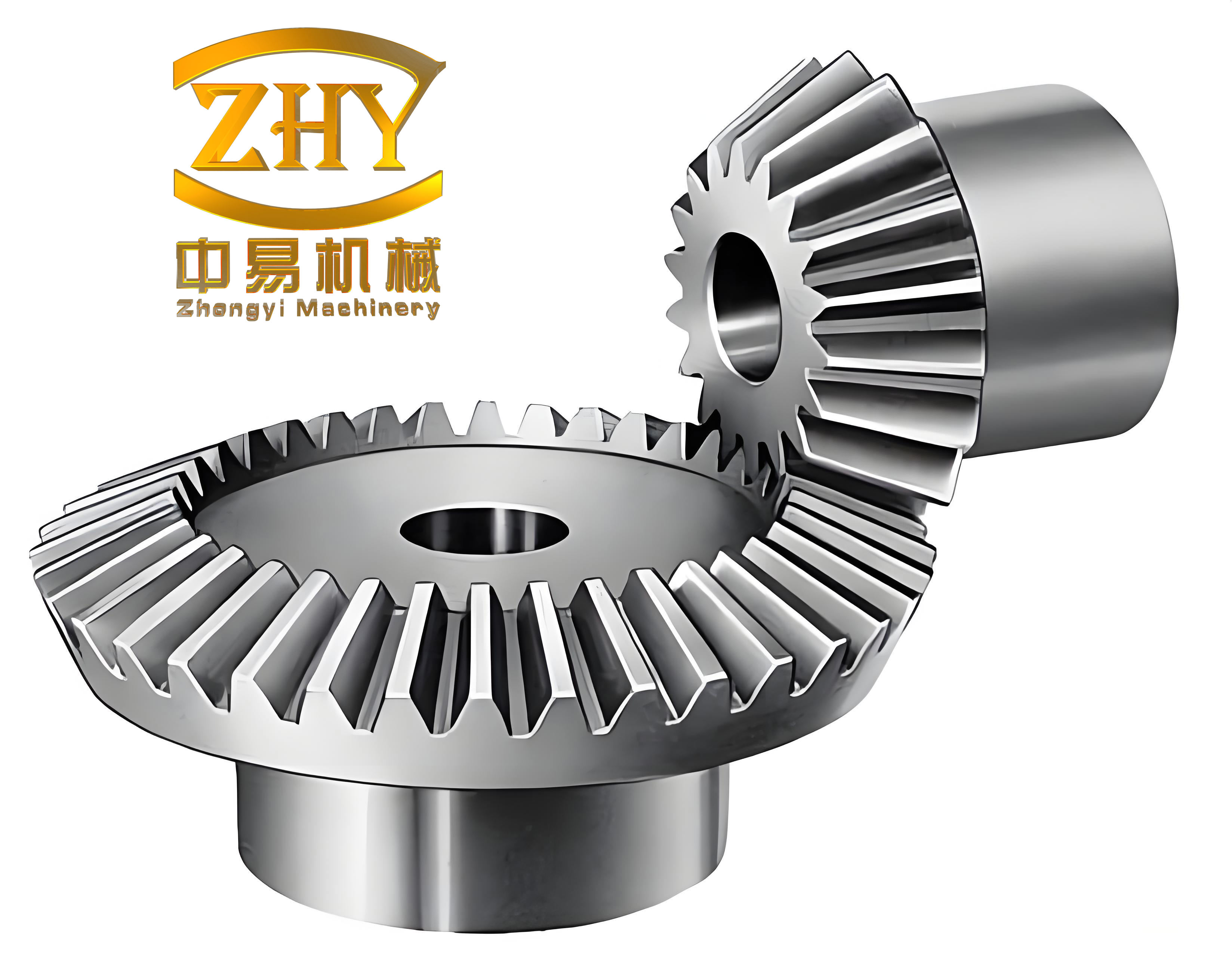
I begin with the geometric meaning of the tooth-surface normal vector. Let a point on a tooth surface be denoted by \(M\). Let the normal line through \(M\) intersect the pitch cone of the straight bevel gear at the node \(O_m\). The length from \(O_m\) to \(M\) along that normal line is written as \(l\), and I call it the tooth-surface normal length. At \(O_m\), I attach a moving rectangular coordinate system \(O_mx_my_mz_m\) such that the \(z_m\)-axis is parallel to the gear axis and the \(y_m\)-axis is tangent to the pitch cone. The normal vector has three direction angles, denoted by \(\alpha\), \(\beta\), and \(\gamma\). The relation between these angles and the geometric parameters of straight bevel gears leads to a compact parameterization.
The unit normal vector of the tooth surface can be written as
$$
\mathbf{n}_l =
\begin{bmatrix}
\sin\beta\cos\lambda \\
\cos\beta \\
-\sin\beta\sin\lambda
\end{bmatrix},
$$
where \(\beta\) is the angle between the normal vector and the \(y_m\)-axis, and \(\lambda\) is an angular parameter describing the orientation of the normal vector around the \(y_m\)-axis. The tooth-surface normal vector itself is therefore
$$
\mathbf{l} = l\mathbf{n}_l =
\begin{bmatrix}
l\sin\beta\cos\lambda \\
l\cos\beta \\
-l\sin\beta\sin\lambda
\end{bmatrix},
$$
with the parameter ranges
$$
0 \le \beta \le \pi, \qquad -\pi \le \lambda \le \pi, \qquad l \ge 0.
$$
This representation is important because it treats the normal vector as a fundamental geometric object. For straight bevel gears, the tooth surface is not imposed in advance as a known curve. Instead, the normal vector field is the unknown, and the surface follows from it. This is what makes the method general and suitable for active design of straight bevel gears.
| Symbol | Meaning | Typical domain |
|---|---|---|
| \(M\) | Point on the tooth surface | Surface point |
| \(O_m\) | Node on the pitch cone where the normal line intersects | Pitch-cone point |
| \(\mathbf{l}\) | Tooth-surface normal vector | Vector field |
| \(l\) | Normal length, \(l = |\mathbf{l}|\) | \(l \ge 0\) |
| \(\mathbf{n}_l\) | Unit normal vector | \(|\mathbf{n}_l| = 1\) |
| \(\alpha,\beta,\gamma\) | Direction angles of the normal vector | \(0 \le \beta \le \pi\) |
| \(\lambda\) | Angular orientation parameter of the normal vector | \(-\pi \le \lambda \le \pi\) |
| \(\phi\) | Rotational parameter of the moving coordinate system | Angular coordinate |
| \(u\) | Axial translation parameter | Axial coordinate |
| \(\delta\) | Pitch cone angle | \(0 < \delta < \pi/2\) |
| \(\delta_b\) | Base cone angle for spherical involute straight bevel gears | \(0 < \delta_b < \delta\) |
I now introduce the coordinate systems that support the generation of straight bevel gears. The fixed coordinate system \(Oxyz\) is attached to the gear blank. A parallel translated coordinate system \(O_tx_ty_tz_t\) is separated from \(Oxyz\) by the axial distance \(u\), so that \(u = OO_t\). Two moving coordinate systems are also used. The system \(O_mx_my_mz_m\) rotates with the tooth-generation parameter \(\phi\), and the system \(O_nx_ny_nz_n\) has an origin coincident with that of \(O_mx_my_mz_m\) but remains parallel to the fixed coordinate axes during motion. In the moving system \(O_mx_my_mz_m\), the \(y_m\)-axis remains tangent to the pitch cone of the straight bevel gear.
Using these definitions, the position vector of a point on the tooth surface in the fixed system \(Oxyz\) is
$$
\mathbf{R}(\phi,u)
=
M_{nm}(\phi)\mathbf{l}
+
M_{tn}(r)
+
M_{st}(u),
$$
where \(M_{nm}(\phi)\) is the rotation matrix from \(O_mx_my_mz_m\) to \(O_nx_ny_nz_n\), \(M_{tn}(r)\) is the translation from \(O_nx_ny_nz_n\) to \(O_tx_ty_tz_t\), and \(M_{st}(u)\) is the translation from \(O_tx_ty_tz_t\) to \(Oxyz\). I write these matrices explicitly as
$$
M_{nm}(\phi)
=
\begin{bmatrix}
\sin\phi & -\cos\phi & 0 \\
\cos\phi & \sin\phi & 0 \\
0 & 0 & 1
\end{bmatrix},
$$
$$
M_{tn}(r)
=
\begin{bmatrix}
r\sin\phi \\
r\cos\phi \\
0
\end{bmatrix},
\qquad
M_{st}(u)
=
\begin{bmatrix}
0 \\
0 \\
u
\end{bmatrix}.
$$
The radius \(r\) is related to the axial parameter \(u\) and the pitch cone angle \(\delta\) by
$$
r = u\tan\delta.
$$
The unit normal vector in the fixed coordinate system is obtained by the same rotation:
$$
\mathbf{n} = M_{nm}(\phi)\mathbf{n}_l.
$$
This is the key transformation that allows me to express both the point coordinates and the normal direction of straight bevel gears in a single consistent framework.
| Coordinate system | Role | Motion property |
|---|---|---|
| \(Oxyz\) | Fixed gear coordinate system | Stationary |
| \(O_tx_ty_tz_t\) | Parallel translated system at axial distance \(u\) | Translated along the gear axis |
| \(O_mx_my_mz_m\) | Moving system attached to the pitch-cone node | Rotates with \(\phi\) |
| \(O_nx_ny_nz_n\) | Auxiliary moving system with coincident origin | Keeps axes parallel to fixed axes |
The meshing conditions for straight bevel gears are obtained from the fundamental condition that the relative velocity must be perpendicular to the common normal at the contact point. In the present notation, I impose
$$
\mathbf{R}’_{\phi}\cdot\mathbf{n}=0,
$$
$$
\mathbf{R}’_{u}\cdot\mathbf{n}=0.
$$
Here \(\mathbf{R}’_{\phi}\) and \(\mathbf{R}’_{u}\) are the partial derivatives of the position vector with respect to the parameters \(\phi\) and \(u\). Substituting the position equation into these conditions gives the governing differential relations for the normal vector field of straight bevel gears. After simplification, I obtain
$$
\frac{dl}{d\phi} = r\cos\beta = u\tan\delta\cos\beta,
$$
$$
\frac{dl}{du}
=
\frac{\sin\beta}{\cos\delta}
\sin(\lambda-\delta).
$$
These two equations are the core of the normal-vector method. They relate the normal length \(l\), the direction angle \(\beta\), the orientation angle \(\lambda\), and the two surface parameters \(\phi\) and \(u\). If any one of the functions \(l(\phi,u)\), \(\beta(\phi,u)\), or \(\lambda(\phi,u)\) is prescribed, then the remaining quantities can be determined through the differential relations, and the tooth surface of the straight bevel gear follows directly.
For a systematic solution, I treat \(l\), \(\beta\), and \(\lambda\) as fields on the parameter domain. The compatibility condition between the two mixed partial derivatives must hold. In general form, I require
$$
\frac{\partial}{\partial u}
\left(
u\tan\delta\cos\beta
\right)
=
\frac{\partial}{\partial \phi}
\left(
\frac{\sin\beta}{\cos\delta}
\sin(\lambda-\delta)
\right).
$$
This condition ensures that the surface obtained by integrating the normal-vector field is continuous and well defined. In practice, I can choose a simple design function, such as a constant or polynomial expression, and then solve the compatibility condition for the remaining function. This is precisely how I create new tooth surfaces for straight bevel gears without restricting myself to classical profile curves.
| Unknown field | Role in the method | Design freedom |
|---|---|---|
| \(l(\phi,u)\) | Normal length from pitch-cone node to surface point | Controls radial distance and local position |
| \(\beta(\phi,u)\) | Direction angle of the normal vector | Controls pressure angle and profile curvature |
| \(\lambda(\phi,u)\) | Orientation of the normal vector around the pitch cone | Controls skewness and surface orientation |
| \(\phi\) | Rotational parameter | Angular coordinate along the tooth |
| \(u\) | Axial parameter | Coordinate along the face width |
I can now describe the general solution procedure for straight bevel gears. First, I define the pitch cone angle \(\delta\), the tooth number, the pressure angle, and the desired face width. Second, I select a design function for one of the three fields \(l\), \(\beta\), or \(\lambda\). Third, I solve the compatibility condition and integrate the differential relations. Fourth, I transform the resulting normal length and direction angles into Cartesian coordinates using the rotation and translation matrices. Fifth, I compute the unit normal vector at every sampled point. Sixth, I generate a discrete surface mesh or a solid model of the straight bevel gear tooth. This procedure is general, and it can be applied to arbitrary tooth profiles as long as the normal-vector field is consistent.
For a direct integration, I write the normal length as
$$
l(\phi,u)
=
l_0
+
\int_0^\phi u\tan\delta\cos\beta(\xi,u)\,d\xi
+
\int_0^u
\frac{\sin\beta(\phi,\eta)}{\cos\delta}
\sin(\lambda(\phi,\eta)-\delta)\,d\eta.
$$
This expression shows that the normal length is obtained from the direction fields. The first integral accumulates the rotational contribution, and the second integral accumulates the axial contribution. In many design problems, I simplify the calculation by choosing either \(\beta\) or \(\lambda\) as a primary design function. If \(\beta\) is prescribed, then \(\lambda\) can be solved from the compatibility condition. If \(\lambda\) is prescribed, then \(\beta\) can be solved from the same condition. If \(l\) is prescribed, then the direction fields must satisfy the two differential relations simultaneously. This flexibility is a major advantage for the active design of straight bevel gears.
| Step | Operation | Output |
|---|---|---|
| 1 | Define the geometric parameters of the straight bevel gear | Pitch cone angle, tooth number, pressure angle, face width |
| 2 | Select a design function for \(l\), \(\beta\), or \(\lambda\) | Primary normal-vector field |
| 3 | Apply the compatibility condition | Consistent secondary field |
| 4 | Integrate the differential relations | Normal length and direction angles on the parameter grid |
| 5 | Use the coordinate transformation | Point coordinates \(\mathbf{R}(\phi,u)\) |
| 6 | Compute the normal vector in the fixed frame | Unit normal field \(\mathbf{n}(\phi,u)\) |
| 7 | Build the surface mesh or solid model | Tooth surface of the straight bevel gear |
A classical and important special case is the spherical involute tooth surface of straight bevel gears. For this case, I let the base cone angle be \(\delta_b\). The spherical involute relation gives
$$
\psi = \phi\sin\delta_b,
$$
and the normal length becomes
$$
l = \frac{u}{\cos\delta}\sin(\phi\sin\delta_b).
$$
Substituting this into the differential relations leads to the direction-angle equations
$$
\cos\beta
=
\frac{\sin\delta_b}{\sin\delta}
\cos(\phi\sin\delta_b),
$$
$$
\sin(\lambda-\delta)
=
\frac{\sin(\phi\sin\delta_b)}{\sin\beta}.
$$
These equations recover the spherical involute geometry of straight bevel gears within the normal-vector framework. I emphasize that I do not need to begin with a spherical involute curve. Instead, the spherical involute appears naturally when I choose the corresponding normal length function. This confirms that the method contains the classical involute solution as a special case while remaining open to many other profile forms.
| Spherical involute quantity | Expression | Interpretation |
|---|---|---|
| \(\psi\) | \(\psi = \phi\sin\delta_b\) | Spherical involute angle |
| \(l\) | \(l = \frac{u}{\cos\delta}\sin(\phi\sin\delta_b)\) | Normal length |
| \(\cos\beta\) | \(\frac{\sin\delta_b}{\sin\delta}\cos(\phi\sin\delta_b)\) | Normal direction angle |
| \(\sin(\lambda-\delta)\) | \(\frac{\sin(\phi\sin\delta_b)}{\sin\beta}\) | Normal orientation angle |
| Surface point | \(\mathbf{R}(\phi,u)\) | Spherical involute tooth surface |
I also apply the method to straight bevel gears whose tooth surfaces are not involute. A convenient design choice is a bivariate polynomial for the direction angle \(\beta(\phi,u)\). I write
$$
\beta(\phi,u)
=
a_0
+
a_1u
+
a_2\phi
+
a_3u\phi
+
a_4u^2
+
a_5\phi^2
+
a_6u^2\phi
+
a_7u\phi^2
+
\cdots .
$$
The coefficients \(a_0,a_1,a_2,\dots\) are design constants. By changing these coefficients, I change the normal-vector field, and therefore I change the tooth surface of the straight bevel gear. This is a direct active-design mechanism. For example, a constant direction angle produces a regular and predictable surface. A linear axial term produces a gradual change along the face width. A linear angular term produces a progressive change along the rotational direction. Higher-order terms allow local modifications of curvature and contact behavior.
| Design case | Direction-angle function | Effect on straight bevel gears |
|---|---|---|
| Constant | \(\beta = a_0\) | Uniform normal direction |
| Linear axial | \(\beta = a_0 + a_1u\) | Gradual variation along the face width |
| Linear angular | \(\beta = a_0 + a_2\phi\) | Progressive variation along the tooth rotation |
| Bilinear | \(\beta = a_0 + a_1u + a_2\phi + a_3u\phi\) | Coupled axial-angular control |
| Quadratic | \(\beta = a_0 + a_1u + a_2\phi + a_4u^2 + a_5\phi^2\) | Local curvature adjustment |
For a numerical example, I consider a straight bevel gear with pitch cone angle \(\delta = 5\pi/36\), which is \(25^\circ\), and tooth number \(z = 18\). I set the pressure-angle reference to \(\pi/9\), which is \(20^\circ\). For the polynomial direction-angle design, I choose a baseline value \(a_0 = 0.349\). I then examine three cases: a constant field, a linear axial field, and a linear angular field. The constant case uses \(a_1 = a_2 = a_3 = 0\). The linear axial case uses \(a_1 = 0.01\), \(a_2 = a_3 = 0\). The linear angular case uses \(a_2 = 0.3\), \(a_1 = a_3 = 0\). Although the numerical changes appear small, the resulting tooth surfaces of the straight bevel gears differ in shape, contact orientation, and local curvature.
| Case | \(a_0\) | \(a_1\) | \(a_2\) | \(a_3\) | Direction-angle function |
|---|---|---|---|---|---|
| Constant | 0.349 | 0 | 0 | 0 | \(\beta = 0.349\) |
| Linear axial | 0.349 | 0.01 | 0 | 0 | \(\beta = 0.349 + 0.01u\) |
| Linear angular | 0.349 | 0 | 0.3 | 0 | \(\beta = 0.349 + 0.3\phi\) |
| Bilinear | 0.349 | 0.01 | 0.3 | 0.02 | \(\beta = 0.349 + 0.01u + 0.3\phi + 0.02u\phi\) |
After choosing the direction-angle function, I solve for \(\lambda\) and \(l\) on a discrete grid. Let the rotational parameter be sampled as \(\phi_i\) and the axial parameter as \(u_j\). For each grid point, I evaluate \(\beta(\phi_i,u_j)\). Then I apply the compatibility condition and the differential relations. The normal length is integrated from the pitch-cone node outward. The surface point is then computed as
$$
\mathbf{R}_{ij}
=
M_{nm}(\phi_i)\mathbf{l}_{ij}
+
M_{tn}(r_j)
+
M_{st}(u_j),
$$
where
$$
\mathbf{l}_{ij}
=
l_{ij}
\begin{bmatrix}
\sin\beta_{ij}\cos\lambda_{ij} \\
\cos\beta_{ij} \\
-\sin\beta_{ij}\sin\lambda_{ij}
\end{bmatrix}.
$$
The corresponding normal vector in the fixed frame is
$$
\mathbf{n}_{ij}
=
M_{nm}(\phi_i)
\begin{bmatrix}
\sin\beta_{ij}\cos\lambda_{ij} \\
\cos\beta_{ij} \\
-\sin\beta_{ij}\sin\lambda_{ij}
\end{bmatrix}.
$$
These discrete points and normals form the basis for the three-dimensional model of the straight bevel gear tooth. I can export the mesh to a computer-aided design environment, fit smooth surface patches, or use the normals for contact analysis. Because the normal vector is computed directly, the surface and its normal field are consistent by construction. This is a significant practical benefit for straight bevel gears, where the contact pattern is highly sensitive to normal direction and curvature.
| Computed quantity | Expression | Use |
|---|---|---|
| \(\beta_{ij}\) | Design function evaluated at \((\phi_i,u_j)\) | Normal direction angle |
| \(\lambda_{ij}\) | Solved from compatibility | Normal orientation angle |
| \(l_{ij}\) | Integrated normal length | Surface position along the normal |
| \(\mathbf{l}_{ij}\) | \(l_{ij}\mathbf{n}_{l,ij}\) | Normal vector before rotation |
| \(\mathbf{R}_{ij}\) | \(M_{nm}\mathbf{l}_{ij}+M_{tn}+M_{st}\) | Surface point |
| \(\mathbf{n}_{ij}\) | \(M_{nm}\mathbf{n}_{l,ij}\) | Surface normal in fixed frame |
The normal-vector method also provides a simple route to check surface quality. I can verify that the computed normal vector is orthogonal to the two tangent vectors obtained by differentiating the position vector. That is, for every sampled point, I check
$$
\frac{\partial\mathbf{R}}{\partial\phi}\cdot\mathbf{n}=0,
$$
$$
\frac{\partial\mathbf{R}}{\partial u}\cdot\mathbf{n}=0.
$$
In an exact solution, these residuals vanish. In a numerical solution, their magnitudes indicate the integration and interpolation error. I can reduce the error by refining the parameter grid, using higher-order integration, or enforcing the compatibility condition more accurately. This kind of self-check is valuable for straight bevel gears because it links the geometry, the normal field, and the meshing condition in one formulation.
| Residual | Exact condition | Numerical target |
|---|---|---|
| \(R_{\phi}\) | \(\mathbf{R}’_{\phi}\cdot\mathbf{n}=0\) | Close to zero |
| \(R_{u}\) | \(\mathbf{R}’_{u}\cdot\mathbf{n}=0\) | Close to zero |
| Compatibility | Mixed derivative equality | Close to zero |
| Unit normal | \(|\mathbf{n}|=1\) | Exactly one |
| On-surface condition | Point lies on generated tooth surface | Consistent by construction |
I can also express the local differential geometry of straight bevel gears through the first and second fundamental forms. Let the two tangent vectors be
$$
\mathbf{R}_{\phi} = \frac{\partial\mathbf{R}}{\partial\phi},
\qquad
\mathbf{R}_{u} = \frac{\partial\mathbf{R}}{\partial u}.
$$
The coefficients of the first fundamental form are
$$
E = \mathbf{R}_{\phi}\cdot\mathbf{R}_{\phi},
\qquad
F = \mathbf{R}_{\phi}\cdot\mathbf{R}_{u},
\qquad
G = \mathbf{R}_{u}\cdot\mathbf{R}_{u}.
$$
The unit normal is already available from the normal-vector method. The second fundamental form coefficients are
$$
L = \mathbf{R}_{\phi\phi}\cdot\mathbf{n},
\qquad
M = \mathbf{R}_{\phi u}\cdot\mathbf{n},
\qquad
N = \mathbf{R}_{uu}\cdot\mathbf{n}.
$$
The Gaussian curvature and mean curvature follow as
$$
K = \frac{LN-M^2}{EG-F^2},
$$
$$
H = \frac{EN-2FM+GL}{2(EG-F^2)}.
$$
These quantities are useful for evaluating the contact behavior of straight bevel gears. Since the normal vector is a primary variable in my method, the second fundamental form can be computed without first fitting an implicit surface. This makes the method attractive for design optimization and for comparing different tooth-profile strategies in straight bevel gears.
| Differential-geometry quantity | Formula | Relevance to straight bevel gears |
|---|---|---|
| \(E\) | \(\mathbf{R}_{\phi}\cdot\mathbf{R}_{\phi}\) | Angular metric |
| \(F\) | \(\mathbf{R}_{\phi}\cdot\mathbf{R}_{u}\) | Coupling metric |
| \(G\) | \(\mathbf{R}_{u}\cdot\mathbf{R}_{u}\) | Axial metric |
| \(L\) | \(\mathbf{R}_{\phi\phi}\cdot\mathbf{n}\) | Curvature in the angular direction |
| \(M\) | \(\mathbf{R}_{\phi u}\cdot\mathbf{n}\) | Twist coupling |
| \(N\) | \(\mathbf{R}_{uu}\cdot\mathbf{n}\) | Curvature in the axial direction |
| \(K\) | \((LN-M^2)/(EG-F^2)\) | Gaussian curvature |
| \(H\) | \((EN-2FM+GL)/(2(EG-F^2))\) | Mean curvature |
The connection between the normal-vector method and the classical meshing condition can be summarized as follows. The tooth surface of a straight bevel gear is generated by a moving point whose normal line always intersects the pitch cone at the node. The normal length and direction angles are not arbitrary; they must satisfy the two meshing differential equations. Once those equations are satisfied, the surface is conjugate to the mating surface in the kinematic sense. This is why the method can generate valid straight bevel gears without explicitly constructing a cutter profile. The cutter or generating curve is effectively replaced by the normal-vector field.
I find that this viewpoint is particularly useful for active design. In conventional practice, a designer chooses a profile curve, such as a spherical involute or a circular arc, and then derives the tooth surface. In my method, the designer chooses a normal-vector field instead. The normal field directly controls the pressure angle, the contact normal, and the local curvature of the straight bevel gears. This means that the design intent can be expressed in terms of contact and normal behavior rather than in terms of a geometric curve that may be difficult to modify.
| Design viewpoint | Primary input | Resulting tooth surface |
|---|---|---|
| Classical profile-curve approach | Spherical involute or circular arc | Fixed family of straight bevel gears |
| Normal-vector approach | \(l\), \(\beta\), or \(\lambda\) field | General and actively designed straight bevel gears |
| Hybrid approach | Profile curve plus normal constraints | Controlled modification of straight bevel gears |
For spherical involute straight bevel gears, I can recover the classical solution by inserting the spherical involute relations into the general equations. This is a useful validation. I choose the base cone angle \(\delta_b\), compute \(\psi = \phi\sin\delta_b\), and then evaluate \(l\), \(\beta\), and \(\lambda\). The resulting surface points and normals satisfy the meshing equations. If I compare the generated surface with an independently constructed spherical involute model, the geometric agreement should be close, apart from numerical discretization. This confirms that the normal-vector method is consistent with established geometry while also being more general.
| Validation item | Method | Expected result |
|---|---|---|
| Spherical involute recovery | Insert \(\psi = \phi\sin\delta_b\) into the general equations | Classical involute surface |
| Normal orthogonality | Check \(\mathbf{R}’_{\phi}\cdot\mathbf{n}\) and \(\mathbf{R}’_{u}\cdot\mathbf{n}\) | Zero residuals |
| Meshing condition | Check the two differential equations | Satisfied |
| Surface continuity | Check compatibility condition | Satisfied |
| CAD consistency | Compare mesh with solid model | Closed and smooth tooth form |
For polynomial straight bevel gears, I use the same validation steps. The difference is that the direction-angle function is no longer tied to the spherical involute. Instead, I choose a polynomial and solve the compatibility condition. The resulting tooth surface may have a pressure angle that varies along the tooth. It may also have a contact normal that changes gradually across the face width. These variations can be used to tune the contact pattern, reduce edge contact, or modify the transmission error of the straight bevel gears. The numerical examples show that small changes in the polynomial coefficients produce visible changes in tooth shape.
In a practical computational workflow, I discretize the parameter domain as
$$
\phi_i = \phi_0 + i\Delta\phi,
\qquad
i=0,1,\dots,N_{\phi},
$$
$$
u_j = u_0 + j\Delta u,
\qquad
j=0,1,\dots,N_{u}.
$$
At each grid point, I compute the normal-vector parameters, transform them into the fixed coordinate system, and store the position and normal. The mesh can then be triangulated or converted into non-uniform rational basis spline patches. For straight bevel gears, I usually refine the grid near the tooth root and near the tooth tip, because those regions often exhibit the largest curvature changes. I also refine the grid near the pitch cone, because the normal length and direction angles vary rapidly there.
| Grid parameter | Typical choice | Reason |
|---|---|---|
| \(N_{\phi}\) | 80 to 300 | Resolve angular variation along the tooth |
| \(N_{u}\) | 40 to 200 | Resolve axial variation across the face width |
| \(\Delta\phi\) | Non-uniform | Refine near pitch cone and tooth edges |
| \(\Delta u\) | Non-uniform | Refine near root and tip regions |
| Integration order | Fourth-order Runge-Kutta or higher | Improve normal-length accuracy |
The numerical integration of the normal length deserves special attention. The differential equation for \(l\) with respect to \(\phi\) and \(u\) is coupled. I can integrate along one parameter direction and then correct along the other direction. A simple and robust approach is to integrate first along \(\phi\) for each fixed \(u\), and then along \(u\) for each fixed \(\phi\). The compatibility condition ensures that the order of integration does not change the final surface, provided the numerical error is controlled. I can also solve the pair of differential equations as a system using a two-dimensional marching scheme.
There are several sources of numerical error. The first is the discretization of the parameter domain. The second is the interpolation of the direction-angle function. The third is the integration scheme. The fourth is the transformation from the moving frame to the fixed frame. I can estimate the total error by evaluating the meshing residuals at the grid points and at midpoints. If the residuals are not sufficiently small, I refine the grid or increase the integration order. This error control is straightforward because the normal-vector equations are explicit and local.
| Error source | Control strategy | Effect on straight bevel gears |
|---|---|---|
| Parameter discretization | Increase grid density | Reduces geometric deviation |
| Direction-angle interpolation | Use higher-order interpolation | Smoothes normal variation |
| Integration scheme | Use Runge-Kutta or spectral methods | Improves normal-length accuracy |
| Coordinate transformation | Use normalized rotation matrices | Preserves orthogonality |
| Surface fitting | Use least-squares or spline fitting | Produces smooth CAD surfaces |
I also consider the role of the pitch cone angle \(\delta\). For straight bevel gears, \(\delta\) determines the relation between the axial parameter \(u\) and the pitch radius \(r = u\tan\delta\). A larger pitch cone angle produces a flatter pitch cone and a different distribution of the normal length. A smaller pitch cone angle produces a steeper pitch cone and a more pronounced variation of the tooth surface along the axial direction. In the normal-vector formulation, \(\delta\) appears explicitly in the differential equations, so its influence is easy to analyze.
| Pitch cone angle | Geometric effect | Normal-vector consequence |
|---|---|---|
| Small \(\delta\) | Steep pitch cone | Strong axial variation of \(l\) |
| Moderate \(\delta\) | Balanced cone | Moderate coupling between \(\phi\) and \(u\) |
| Large \(\delta\) | Flat pitch cone | Weak axial variation of \(l\) |
The method also allows me to study the influence of the base cone angle \(\delta_b\) for spherical involute straight bevel gears. The base cone angle controls the spherical involute curvature and the pressure angle. In the normal-vector equations, \(\delta_b\) appears inside the trigonometric functions \(\sin(\phi\sin\delta_b)\) and \(\cos(\phi\sin\delta_b)\). A change in \(\delta_b\) changes the normal length and the direction angle \(\beta\). This gives me an analytical handle on the classical involute family of straight bevel gears.
For a general design, I may combine the spherical involute baseline with a polynomial modification. For example, I can write
$$
\beta(\phi,u)
=
\beta_{\text{inv}}(\phi,u)
+
\Delta\beta(\phi,u),
$$
where \(\beta_{\text{inv}}\) is the spherical involute direction angle and \(\Delta\beta\) is a polynomial correction. The correction can be used to modify the contact pattern without changing the overall involute character of the straight bevel gears. This hybrid strategy is attractive because it preserves the proven advantages of involute geometry while adding local design freedom. Similar corrections can be applied to \(l\) or \(\lambda\).
| Hybrid design | Base term | Correction term | Purpose |
|---|---|---|---|
| Modified involute \(\beta\) | \(\beta_{\text{inv}}\) | \(\Delta\beta(\phi,u)\) | Adjust contact normal |
| Modified involute \(l\) | \(l_{\text{inv}}\) | \(\Delta l(\phi,u)\) | Adjust local position |
| Modified involute \(\lambda\) | \(\lambda_{\text{inv}}\) | \(\Delta\lambda(\phi,u)\) | Adjust surface orientation |
When I apply the method to the three-dimensional modeling of straight bevel gears, I first generate one tooth surface. Then I mirror or rotate the surface to create the opposite flank. The root and tip are trimmed by the boundary curves obtained from the parameter limits. The tooth is then patterned around the gear axis according to the tooth number \(z\). Because the normal-vector method produces both the surface and its normal, the solid modeling operation can use the normal field for smoothing, offsetting, and contact simulation. This is a practical advantage for straight bevel gears with non-standard profiles.
The normal-vector method also simplifies the calculation of offset surfaces. If I need an offset surface at a distance \(d\) along the normal, I can write
$$
\mathbf{R}_{d}(\phi,u)
=
\mathbf{R}(\phi,u)
+
d\mathbf{n}(\phi,u).
$$
This is useful for defining tolerances, coatings, or clearance surfaces in straight bevel gears. Since \(\mathbf{n}\) is computed directly from the normal-vector field, the offset surface is obtained without solving a new surface-generation problem. I can also compute the normal deviation between two candidate surfaces by projecting the difference onto the normal direction. This gives a quantitative measure of profile deviation for straight bevel gears.
| Operation | Formula | Application |
|---|---|---|
| Offset surface | \(\mathbf{R}_{d} = \mathbf{R} + d\mathbf{n}\) | Clearance and tolerance surfaces |
| Normal deviation | \(\Delta = (\mathbf{R}_2-\mathbf{R}_1)\cdot\mathbf{n}\) | Profile error evaluation |
| Tangent plane | \(\mathbf{n}\cdot(\mathbf{X}-\mathbf{R})=0\) | Local contact approximation |
| Curvature difference | \(K_2-K_1\) | Contact stress indication |
I have described the method in a general coordinate setting, but the implementation can be simplified for many practical cases. If the direction angle \(\beta\) depends only on \(\phi\), then the axial derivative of \(l\) is still present, and \(\lambda\) must be solved accordingly. If \(\beta\) depends only on \(u\), then the rotational derivative of \(l\) is still present, and \(\lambda\) must be solved as a function of \(\phi\). If both dependencies are weak, then approximate solutions can be obtained by separation of variables. These simplifications are useful for rapid design studies of straight bevel gears.
| Simplified case | Assumption | Solution strategy |
|---|---|---|
| Angular-only \(\beta\) | \(\beta = \beta(\phi)\) | Solve \(\lambda(\phi,u)\) from compatibility |
| Axial-only \(\beta\) | \(\beta = \beta(u)\) | Integrate \(l\) and solve \(\lambda(\phi,u)\) |
| Separable \(\beta\) | \(\beta = \beta_1(\phi)\beta_2(u)\) | Use separated integrals and correction |
| Constant \(\lambda\) | \(\lambda = \lambda_0\) | Solve \(\beta(\phi,u)\) from compatibility |
One of the most important outcomes of my formulation is that it provides a direct link between the normal vector and the active design of straight bevel gears. In a conventional design, the tooth surface is a consequence of a chosen cutter or profile. In my method, the normal vector is the design variable. This reverses the usual logic. I can specify where the contact normal should point, how the pressure angle should vary, and how the normal length should change across the face width. Then I solve for the tooth surface that realizes those specifications. This is a powerful capability for straight bevel gears, especially when the contact pattern must be tailored for a specific application.
I can summarize the main equations of the method in a compact table. The table lists the geometric quantity, its definition, and its role in the generation of straight bevel gears. This summary makes the method easy to implement and easy to compare with other approaches.
| Quantity | Definition | Role |
|---|---|---|
| \(\mathbf{n}_l\) | Unit normal in the moving frame | Direction of the tooth-surface normal |
| \(\mathbf{l}\) | \(l\mathbf{n}_l\) | Normal vector with length |
| \(\mathbf{R}\) | \(M_{nm}\mathbf{l}+M_{tn}+M_{st}\) | Surface point in the fixed frame |
| \(\mathbf{n}\) | \(M_{nm}\mathbf{n}_l\) | Surface normal in the fixed frame |
| \(dl/d\phi\) | \(u\tan\delta\cos\beta\) | Rotational evolution of the normal length |
| \(dl/du\) | \(\frac{\sin\beta}{\cos\delta}\sin(\lambda-\delta)\) | Axial evolution of the normal length |
| Compatibility | Mixed derivative equality | Ensures a valid surface |
| \(\mathbf{R}’_{\phi}\cdot\mathbf{n}=0\) | Meshing condition | Conjugate motion |
| \(\mathbf{R}’_{u}\cdot\mathbf{n}=0\) | Meshing condition | Conjugate motion |
I also compare the normal-vector method with conventional surface-generation approaches for straight bevel gears. The conventional approach usually starts from a generating curve, such as a spherical involute, and then sweeps or rolls that curve according to the gear kinematics. The normal-vector method starts from the normal field and then solves for the surface. The two approaches can produce the same surface when the normal field is chosen consistently with the classical profile. However, the normal-vector method offers more freedom because the normal field can be modified independently of a specific generating curve.
| Criterion | Conventional profile-curve approach | Normal-vector approach |
|---|---|---|
| Primary input | Generating curve | Normal-vector field |
| Design freedom | Limited by curve family | General |
| Involute recovery | Direct | Special case |
| Contact control | Indirect | Direct |
| Numerical implementation | Usually geometric | Differential and algebraic |
| CAD integration | Requires surface fitting | Surface and normal generated together |
The method is not limited to external straight bevel gears. It can also be adapted to internal or crown-like bevel geometries by changing the sign conventions and the coordinate transformations. The main requirement is that the normal line intersects the reference cone at the node and that the meshing conditions are enforced. For straight bevel gears, this geometric condition is natural and leads to a clean formulation. I can therefore use the same equations for a broad class of bevel-type tooth surfaces.
In terms of computational cost, the normal-vector method is efficient. The evaluation of the normal vector and the surface point at one grid point involves only trigonometric functions, matrix-vector products, and simple arithmetic. The integration of the normal length is the most expensive part, but it can be performed with a modest number of steps because the differential equations are smooth. For typical straight bevel gears, a grid of a few hundred points in each parameter direction is sufficient to produce a smooth model. This makes the method suitable for iterative design and optimization.
| Computational task | Operation count per point | Typical cost level |
|---|---|---|
| Evaluate \(\beta,\lambda,l\) | Several trigonometric and arithmetic operations | Low |
| Compute \(\mathbf{l}\) | Three multiplications and three additions | Low |
| Apply \(M_{nm}\) | Nine multiplications and six additions | Low |
| Add translations | Three additions | Low |
| Integrate \(l\) | Depends on integration order and grid size | Moderate |
| Curvature evaluation | Additional derivatives and dot products | Moderate |
I also note that the normal-vector method can be used for reverse engineering. If I have a measured tooth surface of a straight bevel gear, I can estimate the normal vector at each measured point. Then I can fit the direction angles \(\beta\) and \(\lambda\) and the normal length \(l\) as functions of \(\phi\) and \(u\). Once these fields are fitted, I can reconstruct the surface and compare it with a nominal design. This is useful for quality inspection and for understanding the geometric deviations of manufactured straight bevel gears.
For contact analysis, the normal-vector representation is especially convenient. The contact condition between two straight bevel gears can be expressed as the equality of position and the collinearity of normals at the contact point. In my notation, if the two surfaces are \(\mathbf{R}_1\) and \(\mathbf{R}_2\), then at contact I require
$$
\mathbf{R}_1(\phi_1,u_1) = \mathbf{R}_2(\phi_2,u_2),
$$
$$
\mathbf{n}_1(\phi_1,u_1) \parallel \mathbf{n}_2(\phi_2,u_2).
$$
The second condition can be written as
$$
\mathbf{n}_1 \times \mathbf{n}_2 = \mathbf{0}.
$$
Because the normals are generated directly by the method, this contact equation is easy to assemble. I can solve it numerically for the contact parameters and then evaluate the contact ellipse, the transmission error, and the load distribution. This is a strong reason to use the normal-vector method in the design and analysis of straight bevel gears.
| Contact condition | Equation | Purpose |
|---|---|---|
| Position equality | \(\mathbf{R}_1=\mathbf{R}_2\) | Common contact point |
| Normal collinearity | \(\mathbf{n}_1\times\mathbf{n}_2=\mathbf{0}\) | Common tangent plane |
| Meshing condition | \(\mathbf{R}’\cdot\mathbf{n}=0\) | Conjugate motion |
| Transmission error | \(\Delta\theta = \theta_2 – z_2\theta_1/z_1\) | Motion accuracy |
I can also use the normal-vector method to design straight bevel gears with a predetermined pressure-angle distribution. The pressure angle is related to the direction angle \(\beta\). By specifying \(\beta(\phi,u)\), I effectively specify how the pressure angle changes over the tooth surface. This is useful for avoiding undercut, reducing sliding velocity, and improving the contact strength. In the normal-vector formulation, the pressure-angle control is direct and explicit, which is not always the case in conventional profile-based design.
For a practical design study, I might specify a target normal-length function \(l(\phi,u)\) and then solve for \(\beta\) and \(\lambda\). This is the inverse problem of the usual approach. The target normal length can be chosen to control the radial position of the surface, the tooth thickness, and the clearance. The compatibility condition then determines the direction angles. This inverse design capability is one of the main attractions of the method for straight bevel gears.
| Design target | Prescribed function | Solved functions |
|---|---|---|
| Normal-length control | \(l(\phi,u)\) | \(\beta(\phi,u)\), \(\lambda(\phi,u)\) |
| Pressure-angle control | \(\beta(\phi,u)\) | \(l(\phi,u)\), \(\lambda(\phi,u)\) |
| Orientation control | \(\lambda(\phi,u)\) | \(l(\phi,u)\), \(\beta(\phi,u)\) |
The equations also reveal the relationship between the normal length and the geometry of the pitch cone. The term \(u\tan\delta\) is the pitch radius at the axial station \(u\). The rotational derivative of the normal length is proportional to this radius and to \(\cos\beta\). The axial derivative is proportional to \(\sin\beta\) and to \(\sin(\lambda-\delta)\). Therefore, the normal length changes most rapidly when the normal vector is strongly aligned with the corresponding parameter direction. This insight can guide the choice of the design functions for straight bevel gears.
I can also derive a dimensionless form of the differential equations. Let
$$
\bar{l} = \frac{l}{u_0},
\qquad
\bar{u} = \frac{u}{u_0},
$$
where \(u_0\) is a reference axial length. Then the equations become
$$
\frac{d\bar{l}}{d\phi}
=
\bar{u}\tan\delta\cos\beta,
$$
$$
\frac{d\bar{l}}{d\bar{u}}
=
\frac{\sin\beta}{\cos\delta}
\sin(\lambda-\delta).
$$
This dimensionless form is convenient for comparing different sizes of straight bevel gears. It shows that the geometry scales with \(u_0\), while the direction angles remain unchanged. This scaling property is useful for parametric design and for creating families of straight bevel gears with similar contact characteristics.
| Dimensionless quantity | Definition | Benefit |
|---|---|---|
| \(\bar{l}\) | \(l/u_0\) | Scale-independent normal length |
| \(\bar{u}\) | \(u/u_0\) | Scale-independent axial coordinate |
| \(\beta\) | Angle | Already dimensionless |
| \(\lambda\) | Angle | Already dimensionless |
| \(\delta\) | Angle | Already dimensionless |
I have found that the normal-vector method is especially suitable for generating families of straight bevel gears with controlled variations. By changing a single coefficient in the polynomial for \(\beta\), I can produce a family of surfaces that share the same basic geometry but differ in local contact behavior. This is valuable for optimization, where many design candidates must be evaluated quickly. The method avoids the need to reconstruct a generating curve for each candidate, because the normal field itself is the design variable.
In a manufacturing context, the generated tooth surfaces can be used to define cutter paths or grinding paths for straight bevel gears. The normal field provides the tool orientation at each point, which is essential for five-axis machining or for profile grinding. Because the surface and normal are computed together, the tool path generation becomes more direct. I can offset the surface along the normal to account for tool radius, and I can use the normal to control the tool axis orientation. This is another practical benefit of the method.
| Manufacturing task | Information from the method | Use |
|---|---|---|
| Cutter path | Surface points \(\mathbf{R}\) | Define tool tip trajectory |
| Tool orientation | Normal vector \(\mathbf{n}\) | Control tool axis |
| Offset compensation | \(\mathbf{R}+d\mathbf{n}\) | Account for tool radius |
| Inspection | Normal deviation | Compare with nominal straight bevel gears |
The method also offers a clear path to sensitivity analysis. If a design coefficient \(a_k\) changes, the direction angle \(\beta\) changes, and this change propagates to \(\lambda\), \(l\), \(\mathbf{R}\), and \(\mathbf{n}\). I can compute the sensitivity derivatives analytically or numerically. For straight bevel gears, this helps identify which coefficients have the strongest influence on contact position and curvature. The designer can then focus on the most effective parameters. This is an efficient way to optimize straight bevel gears with non-standard tooth surfaces.
I can express the sensitivity of the surface point with respect to a design parameter \(p\) as
$$
\frac{\partial\mathbf{R}}{\partial p}
=
M_{nm}
\frac{\partial\mathbf{l}}{\partial p}
+
\frac{\partial M_{nm}}{\partial p}\mathbf{l}
+
\frac{\partial M_{tn}}{\partial p}
+
\frac{\partial M_{st}}{\partial p}.
$$
If \(p\) only affects the direction angles, then the translation terms vanish, and the sensitivity is determined by the normal-vector derivatives. The normal sensitivity is
$$
\frac{\partial\mathbf{n}}{\partial p}
=
M_{nm}
\frac{\partial\mathbf{n}_l}{\partial p}
+
\frac{\partial M_{nm}}{\partial p}\mathbf{n}_l.
$$
These expressions are useful for gradient-based optimization of straight bevel gears. They are straightforward to implement because the normal vector is already an explicit function of the design parameters.
| Sensitivity | Expression | Design use |
|---|---|---|
| \(\partial\mathbf{R}/\partial p\) | Derivative of the surface point | Shape optimization |
| \(\partial\mathbf{n}/\partial p\) | Derivative of the normal | Contact optimization |
| \(\partial l/\partial p\) | Derivative of normal length | Position control |
| \(\partial\beta/\partial p\) | Derivative of direction angle | Pressure-angle control |
| \(\partial\lambda/\partial p\) | Derivative of orientation angle | Skew control |
In summary, I have presented a normal-vector method for the tooth surfaces of straight bevel gears. The method uses the normal length and the direction angles of the tooth-surface normal as primary variables. The position of the surface is obtained by a sequence of coordinate transformations. The meshing conditions reduce to two differential relations for the normal length. These relations contain the pitch cone angle, the direction angle, and the orientation angle. By choosing one of these functions, I can generate a wide variety of tooth surfaces for straight bevel gears. The spherical involute surface appears as a special case, and polynomial surfaces can be designed actively. The method is general, computationally practical, and well suited to three-dimensional modeling, contact analysis, and manufacturing of straight bevel gears.
I conclude that the normal-vector approach provides a coherent framework for the geometry of straight bevel gears. It does not replace the classical theory; rather, it embeds the classical theory in a broader design space. The normal vector is the natural carrier of contact information, and by making it the primary unknown, I obtain a direct and flexible method for generating tooth surfaces. For straight bevel gears with spherical involute profiles, the method reproduces the expected geometry. For straight bevel gears with polynomial or hybrid profiles, the method opens new possibilities for active design. I expect this formulation to be useful for researchers and engineers who need to create, analyze, and optimize straight bevel gears beyond the standard profile families.