
I investigate a non-uniform meshing strategy for improving the accuracy of gear shaping when the available machine tool, inspection system, and control platform are already fixed. The central problem is practical: conventional gear shaping can usually reach a moderate industrial accuracy level, but many modern transmission systems require pitch accumulation and runout performance that is close to the highest production grades. The difficulty is amplified when the workpiece family includes internal gears, eccentric gears, sector gears, and gears with short cutter relief grooves, because many of these geometries cannot be finished efficiently on a conventional gear grinding machine. I therefore treat the gear shaping process itself as the accuracy-improvement space. Instead of attempting to rebuild the machine tool, I combine full-coordinate error evaluation, data-enhanced long short-term memory prediction, error decoupling, and a non-uniform meshing tool path so that the existing machine can produce a better gear from the same class of forged gear blanks.
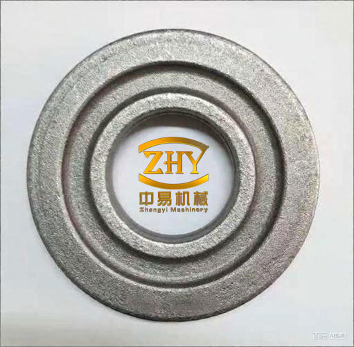
The incoming forged gear blanks are important to this study because they define the physical boundary of the process. The forged gear blanks are not ideal artifacts; they carry lot-to-lot variation, residual surface conditions, and minor geometric deviations that affect the first cutting passes. I do not assume that the forged gear blanks are identical. Instead, I use the error history of previously machined workpieces to predict the error tendency of the next workpiece and to adjust the tool radial feed and tool rotation parameters before cutting. This is the reason the method is described as a pre-compensation method rather than a post-process correction method. The same forged gear blanks can therefore be machined with a non-uniform meshing path that responds to the predicted pitch accumulation and runout behavior.
I organize the work around four technical questions. First, how do the radial feed axis, tool rotation axis, and workpiece rotation axis map to the gear pitch accumulation total deviation and the gear ring radial runout tolerance. Second, how can the tooth flank be evaluated from full-coordinate measurement data instead of a small number of pitch-circle points. Third, how can the time-ordered error records from forged gear blanks be used to predict the error of the next workpiece. Fourth, how can the predicted error be decoupled into machine-axis adjustments and converted into a non-uniform meshing path that remains kinematically stable. The following sections answer these questions with mathematical models, tables, simulation checks, and machining experiments.
Process Model and Error Mapping
I reduce the four-axis CNC gear shaping system to the three axes that dominate the target accuracy indices: the tool radial feed axis X, the tool rotation axis Ct, and the workpiece rotation axis Cw. The main reciprocating axis is not ignored in the physical machine, but its dominant influence is on the lead or helix direction rather than on the pitch accumulation and ring runout investigated here. The coordinate systems are defined so that the tool coordinate frame rotates with the cutter and the workpiece coordinate frame rotates with the workpiece. The nominal center distance is a, the workpiece module is m, the workpiece tooth number is z, the tool module is mt, the tool tooth number is zt, and the pressure angles are α and αt. The nominal transmission ratio is kept constant in the conventional process, while the non-uniform process introduces controlled variation around the nominal ratio.
| Symbol | Meaning | Role in the model |
|---|---|---|
| X | Tool radial feed axis | Controls center-distance variation and radial penetration |
| Ct | Tool rotation axis | Controls cutter angular position and cutter-side generating motion |
| Cw | Workpiece rotation axis | Controls workpiece angular position and generating motion |
| a | Center distance | Defines the relative position of cutter and workpiece |
| m, z | Workpiece module and tooth number | Define nominal pitch radius and pitch |
| mt, zt | Tool module and tooth number | Define cutter geometry and angular compensation |
| α, αt | Pressure angles | Project axis errors onto the mesh line |
| δX | Radial feed error | Produces normal and tangential components |
| δθt, δθw | Angular errors of tool and workpiece | Produce angular and linear error components |
| Fp | Total pitch accumulation deviation | Primary accuracy index in the circumferential direction |
| Fr | Ring radial runout tolerance | Primary accuracy index in the radial direction |
I model the grid of generating positions as a sequence of nominal mesh points and actual mesh points. At each cutting position, the cutter edge removes material at a point that is slightly displaced from the theoretical mesh point because the three controlled axes carry small tracking errors. The projection of these errors onto the normal direction of the tooth profile produces profile deviation, the projection onto the pitch-circle tangent produces pitch accumulation, and the projection onto the radial direction produces ring runout. The coefficients are not identical because the geometric projection depends on the pressure angle and on the local direction of the mesh line.
For the tooth profile deviation, I write the mapped error as
$$
\delta f=\lambda_X\delta X\sin\alpha+
\lambda_w\frac{\pi m z\cos\alpha}{360}\delta\theta_w+
\lambda_t\frac{\pi m_t z_t\cos\alpha_t}{360}\delta\theta_t .
$$
For the total pitch accumulation deviation, the radial feed error is projected through the tangent direction, and the angular errors are converted into arc-length errors on the pitch circle. The resulting model is
$$
F_p=\lambda_X\delta X\tan\alpha+
\lambda_w\frac{\pi m z\cos\alpha}{360}\delta\theta_w+
\lambda_t\frac{\pi m_t z_t\cos\alpha_t}{360}\delta\theta_t .
$$
For the ring radial runout tolerance, the radial feed error enters directly, while the angular errors enter through the sine projection. I therefore use
$$
F_r=\lambda_X\delta X+
\lambda_w\frac{\pi m z\sin\alpha}{360}\delta\theta_w+
\lambda_t\frac{\pi m_t z_t\sin\alpha_t}{360}\delta\theta_t .
$$
The sign coefficients λX, λw, and λt take values of either +1 or -1 according to the local cutting direction, the workpiece rotation direction, and the tool rotation direction. Their role is not to change the magnitude of the mapping but to preserve the direction of the compensation. In the practical implementation, I identify the sign from the measured error trend and from the commanded rotation direction, and I keep the sign consistent during one compensation cycle.
| Axis error | Profile deviation contribution | Pitch accumulation contribution | Ring runout contribution |
|---|---|---|---|
| Radial feed error δX | δX sin α | δX tan α | δX |
| Workpiece angular error δθw | (π m z cos α / 360) δθw | (π m z cos α / 360) δθw | (π m z sin α / 360) δθw |
| Tool angular error δθt | (π mt zt cos αt / 360) δθt | (π mt zt cos αt / 360) δθt | (π mt zt sin αt / 360) δθt |
The mapping gives me the bridge between inspection and control. If the predicted pitch accumulation is positive, I reduce the radial feed by the corresponding absolute amount or adjust the tool angular speed in the opposite direction. If the predicted runout is positive, I treat it as a center-distance offset and compensate the radial axis directly. The angular correction is distributed between the tool and workpiece axes, but in this work I keep the workpiece angular speed fixed and assign the compensation to the tool rotation axis. This choice simplifies the numerical control program and reduces the risk of synchronization loss during the generating motion. The same choice is also convenient for the forged gear blanks because it does not require a new fixture or a new workpiece datum for each batch.
Full-Coordinate Error Evaluation
I do not evaluate the gear from one or two points near the pitch circle. The reason is that a single-point measurement can be influenced by local surface topography, residual chips, probe triggering scatter, and the specific location of the selected point. When the measured error is later decoupled into axis corrections, this local scatter can be amplified into an incorrect compensation. I therefore measure the full tooth flank and fit the involute from the measured coordinate cloud. The full-coordinate evaluation is performed on the same forged gear blanks after shaping, and the resulting error records become the input to the prediction model.
The measured points are first converted from Cartesian coordinates to polar coordinates:
$$
\rho^2=x^2+y^2,\qquad x=\rho\cos\theta,\qquad y=\rho\sin\theta .
$$
The radial interval is then restricted so that the addendum region and the root transition region are excluded. For a workpiece with a small tooth number, the base circle may lie outside the root circle; for a workpiece with a larger tooth number, the root circle may lie outside the base circle. I therefore keep only the points whose polar radius lies inside the active involute interval.
| Tooth-number condition | Retained radial interval | Reason |
|---|---|---|
| z ≤ 41 | rb < ρ < ra | The base circle is outside the root circle |
| z ≥ 42 | rf < ρ < ra | The root circle is outside the base circle |
After filtering, the points are separated into left and right flanks of each tooth. For z teeth, this produces 2z groups. I keep the grouping because the left and right flanks of the same forged gear blanks can have different error trends, especially when the blank has a slight asymmetric residual stress distribution. The groups are processed independently so that a local anomaly on one flank does not contaminate the involute position on the other flank.
I remove abnormal points using a chord-distance criterion and a three-sigma rule. For a point Pi, the adjacent points Pi-1 and Pi+1 define a local chord. The distance from Pi to that chord is
$$
d_i=\frac{|A x_i+B y_i+C|}{\sqrt{A^2+B^2}},
$$
where A, B, and C are the coefficients of the line through Pi-1 and Pi+1. The deviation from the local mean chord distance is
$$
\Delta_i=|d_i-\bar d|,\qquad
\sigma=\sqrt{\frac{1}{n}\sum_{i=1}^{n}\Delta_i^2}.
$$
If Δi > 3σ, the point is treated as an outlier and removed. This criterion is simple, but it is effective for the forged gear blanks because it is sensitive to isolated spikes and insensitive to the smooth curvature of the involute. In the measurement sets I processed, the outlier fraction was small, but removing it improved the stability of the subsequent B-spline fit.
I fit a cubic B-spline through four points located nearest to the pitch circle, two below and two above. The local curve is
$$
\begin{aligned}
x(u)&=a_0+a_1u+a_2u^2+a_3u^3,\\
y(u)&=b_0+b_1u+b_2u^2+b_3u^3,
\end{aligned}
\qquad 0\le u\le 1 .
$$
The four control points are ordered along the flank, and the coefficients are obtained from the standard cubic B-spline basis. The intersection of this local curve with the pitch circle gives a reference point P. I use P to anchor a family of involutes whose base radius and starting angle are allowed to vary inside the accuracy interval of the shaping process. The involute is written as
$$
r_k=\frac{r_b}{\cos\alpha_k},\qquad
\theta_k=\tan\alpha_k-\alpha_k,
$$
and in Cartesian form,
$$
\begin{aligned}
x&=r_b(\cos t+t\sin t),\\
y&=r_b(\sin t-t\cos t).
\end{aligned}
$$
The involute generated from the x-axis is rotated so that it passes through P:
$$
\begin{bmatrix}x\\y\end{bmatrix}
=
\begin{bmatrix}\cos\varphi&-\sin\varphi\\
\sin\varphi&\cos\varphi\end{bmatrix}
\begin{bmatrix}x’\\y’\end{bmatrix}.
$$
I then generate an involute family by varying the base radius and the starting angle inside the estimated error interval. For each involute in the family, every measured point is projected onto the curve, and the point-to-curve distance is evaluated. The total distance for the j-th involute is
$$
E_j=\sum_{i=1}^{n}\sqrt{(x_i-x_{ij}^{*})^2+(y_i-y_{ij}^{*})^2},
$$
and the selected involute is
$$
j_{\mathrm{opt}}=\arg\min_j E_j .
$$
This regional traversal is more robust than a direct algebraic solution because it does not depend on a single reference point and it allows the base radius to absorb the small radial trend caused by the machine error. Once the optimal involute is found, the pitch accumulation and the ring runout are computed from its position relative to the nominal geometry. The pitch accumulation is the maximum difference between the actual arc length and the nominal arc length over the tooth sequence:
$$
F_p=\max_{1\le i<j\le $$=""
The ring runout is obtained from the deviation between the optimal base radius and the nominal base radius:
$$
F_r=\left|r_{b,\mathrm{opt}}-r_{b,\mathrm{nom}}\right|.
$$
I compared the full-coordinate evaluation with the conventional single-point evaluation on the same forged gear blanks. The numerical values were close, but the full-coordinate result was more stable from tooth to tooth and provided a per-tooth error curve instead of a single aggregate value. This per-tooth curve is essential for the subsequent prediction step because the LSTM model learns the sequence pattern rather than only the final scalar index.
| Index | Conventional evaluation (mm) | Full-coordinate evaluation (mm) | Observation |
|---|---|---|---|
| Left-flank pitch accumulation | 0.0474 | 0.0417 | Full-coordinate result follows the fitted involute rather than a local point |
| Right-flank pitch accumulation | 0.0399 | 0.0379 | Slightly lower and more consistent with the tooth sequence |
| Ring radial runout | 0.0169 | 0.0185 | Radial trend is captured more completely |
The full-coordinate method also gives a natural way to store the error signature of each forged gear blank. I store the left-flank pitch curve, the right-flank pitch curve, and the runout curve as a three-channel sequence. The sequence is indexed by tooth number and by batch order. This data structure is used directly by the prediction model described in the next section.
Data-Enhanced LSTM Prediction
The error records from forged gear blanks form a time-ordered data set: each new workpiece is machined after the previous one, and the machine thermal state, fixture state, and cutter wear state evolve gradually. A purely static regression model would ignore this order. I therefore use a recurrent model, specifically a long short-term memory network, to learn the sequence dependence. Because the number of complete workpieces in one experimental campaign is limited, I first apply data augmentation. The augmentation does not replace measurement; it interpolates between measured error states so that the network sees a denser representation of the same process trend.
I use two augmentation families. The first is linear interpolation between neighboring error records. If two records are separated by a distance L and n intermediate states are required, the intermediate coordinate is placed at equal intervals along the chord. The second is cubic B-spline interpolation. The B-spline augmentation produces a smoother transition between records and is better suited to the pitch accumulation curve because the curve is continuous but not necessarily linear. I use the B-spline interpolation for the main training set and keep the linear interpolation as a check for over-smoothing.
$$
\begin{aligned}
x(u)&=a_0+a_1u+a_2u^2+a_3u^3,\\
y(u)&=b_0+b_1u+b_2u^2+b_3u^3,
\end{aligned}
\qquad 0\le u\le 1 .
$$
The LSTM cell is governed by the following gate equations:
$$
f_t=\sigma\left(W_f[h_{t-1},x_t]+b_f\right),
$$
$$
i_t=\sigma\left(W_i[h_{t-1},x_t]+b_i\right),
\qquad
\tilde C_t=\tanh\left(W_C[h_{t-1},x_t]+b_C\right),
$$
$$
C_t=f_t\odot C_{t-1}+i_t\odot\tilde C_t,
$$
$$
o_t=\sigma\left(W_o[h_{t-1},x_t]+b_o\right),
\qquad
h_t=o_t\odot\tanh(C_t).
$$
The input to the network is a three-dimensional tensor with batch size, time-step length, and feature dimension. The features are the left-flank pitch error, the right-flank pitch error, the ring runout, and the batch index. The output is the predicted error vector of the next forged gear blank. I normalize each feature channel before training. The loss function is the mean squared error, and the optimizer is Adam. I compare three network structures: a single-layer LSTM, a two-layer LSTM, and a bidirectional LSTM. The comparison is necessary because a deeper or bidirectional model is not automatically better when the data set is small and the process trend is smooth.
| Item | Setting |
|---|---|
| Input features | Left pitch curve, right pitch curve, ring runout, batch index |
| Time-step basis | One machining batch segment |
| Batch size | 5 |
| LSTM output size | 300 |
| First fully connected layer | 1200 neurons |
| Second fully connected layer | 1 neuron |
| Training/test split | 8:2 |
| Activation | Sigmoid and tanh gates |
| Optimizer | Adam |
| Learning rate | 0.005 |
| Epochs | 300 |
The prediction accuracy is quantified with the root mean square error and the mean absolute error:
$$
\mathrm{RMSE}=\sqrt{\frac{1}{N}\sum_{i=1}^{N}\left(\hat y_i-y_i\right)^2},
\qquad
\mathrm{MAE}=\frac{1}{N}\sum_{i=1}^{N}\left|\hat y_i-y_i\right|.
$$
I compared the three models on the same augmented data set. The single-layer LSTM produced the lowest error for all three targets. The two-layer LSTM was smoother but less responsive to the local tooth-to-tooth trend. The bidirectional LSTM showed occasional abrupt changes, which is undesirable for compensation because a single abrupt correction can produce a visible mark on the flank. I therefore selected the single-layer data-enhanced LSTM as the prediction model for the non-uniform meshing path.
| Target | Model | RMSE | MAE |
|---|---|---|---|
| Left-flank pitch accumulation | DA-LSTM | 0.0546 | 0.0624 |
| Left-flank pitch accumulation | DA-TWO-LSTM | 0.0983 | 0.0872 |
| Left-flank pitch accumulation | DA-Bi-LSTM | 0.1479 | 0.1512 |
| Right-flank pitch accumulation | DA-LSTM | 0.0589 | 0.0648 |
| Right-flank pitch accumulation | DA-TWO-LSTM | 0.0920 | 0.0854 |
| Right-flank pitch accumulation | DA-Bi-LSTM | 0.1498 | 0.1473 |
| Ring radial runout | DA-LSTM | 0.0554 | 0.0619 |
| Ring radial runout | DA-TWO-LSTM | 0.0975 | 0.0887 |
| Ring radial runout | DA-Bi-LSTM | 0.1509 | 0.1603 |
The prediction output is not used as a scalar correction. It is used as a tooth-indexed correction curve. For each tooth position, the predicted left pitch error, right pitch error, and runout are converted into a radial correction and an angular correction. This preserves the local information that the full-coordinate evaluation produced and avoids flattening the correction into a single constant offset. The forged gear blanks in the next batch therefore receive a correction that follows the predicted tooth sequence rather than a uniform center-distance shift.
| Tooth index | Left pitch error (mm) | Right pitch error (mm) | Ring runout (mm) |
|---|---|---|---|
| 1 | -0.0095 | -0.0071 | -0.0291 |
| 2 | -0.0148 | -0.0098 | -0.0213 |
| 3 | -0.0134 | -0.0088 | -0.0382 |
| 4 | -0.0124 | -0.0149 | -0.0413 |
| 5 | -0.0080 | -0.0061 | -0.0393 |
| 6 | -0.0076 | -0.0064 | -0.0361 |
| 7 | -0.0063 | -0.0068 | -0.0388 |
| 8 | -0.0084 | 0.0126 | -0.0274 |
| 9 | -0.0078 | -0.0022 | -0.0286 |
Error Decoupling and Non-uniform Meshing Path
The predicted errors are decoupled into the radial feed axis and the tool rotation axis. The workpiece rotation axis is kept at its nominal angular speed to preserve the generating ratio, while the tool rotation axis absorbs the angular part of the correction. For pitch accumulation, the radial component is
$$
\delta X_{Fp}=\frac{F_p}{\tan\alpha},
$$
and the angular speed correction assigned to the tool axis is
$$
\omega_{c}=\frac{360F_p}{\pi m_t z_t\cos\alpha_t}
+
\frac{360F_p}{\pi m z\cos\alpha}.
$$
For ring runout, the radial component is direct:
$$
\delta X_{Fr}=F_r,
$$
and the angular speed correction is
$$
\omega_{r}=\frac{360F_r}{\pi m_t z_t\sin\alpha_t}
+
\frac{360F_r}{\pi m z\sin\alpha}.
$$
The total radial correction is the sum of the pitch and runout contributions, and the total tool angular correction is the sum of the corresponding angular terms. The sign of each term is determined by the direction of the predicted error and by the sign convention of the machine axes. In the numerical control program, the correction is distributed along the generating path as a smooth function of the generating angle rather than as a step change at a single tooth. This is the essential difference between a conventional uniform meshing path and the non-uniform meshing path used here.
| Original X (mm) | Radial correction (mm) | Adjusted X (mm) | Original C2 (deg) | Angular correction (deg) | Adjusted C2 (deg) |
|---|---|---|---|---|---|
| 10.0000 | -0.0198 | 9.9802 | 0.5000 | -0.0409 | 0.5409 |
| 10.0000 | -0.0339 | 9.9661 | 0.5000 | -0.0423 | 0.5423 |
| 10.0000 | -0.0142 | 9.9858 | 0.5000 | -0.0399 | 0.5399 |
| 10.0000 | -0.0162 | 9.9838 | 0.5000 | -0.0396 | 0.5396 |
I express the non-uniform meshing path as a nominal center distance plus a smooth modulation and a nominal tool angle plus a smooth angular modulation:
$$
a(\varphi)=a_0+\delta X_{Fp}\cos\varphi+\delta X_{Fr}\sin\varphi,
$$
$$
\theta_t(\varphi)=\omega_t t+\Delta\theta_t(\varphi).
$$
The modulation is periodic over one workpiece revolution but not constant within a revolution. The cutter therefore experiences a continuously varying center distance and a continuously varying relative meshing position. This is the meaning of non-uniform meshing in this study. It is not a random disturbance. It is a deterministic, error-driven modulation that is generated from the predicted error curve and is synchronized with the generating motion.
The non-uniform path has two practical advantages for forged gear blanks. First, it does not require a new fixture or a new machine configuration. The forged gear blanks are loaded in the same way as in the conventional process. Second, the correction is applied during the generating motion, so the final tooth flank is formed with the corrected relative position instead of being corrected after the tooth flank has already been cut. This is important because a post-process correction would require a second setup and would disturb the datum established from the forged gear blanks.
Simulation and Machining Validation
I first checked the non-uniform path in a virtual machining environment. The simplified machine model contained the radial feed axis, the tool rotation axis, and the workpiece rotation axis. The cutter and the workpiece blank were modeled from the same nominal geometry used in the experiment. The control program was generated from the decoupled correction table, and the virtual machine was run through a complete shaping cycle. The purpose of the simulation was not to predict the final accuracy numerically but to detect interference, axis over-travel, synchronization loss, and abnormal cutter-workpiece engagement. The non-uniform path passed these checks without collision or program error.
I then machined a set of workpieces on the available four-axis CNC gear shaping platform. The forged gear blanks were prepared in the same batch and measured before and after shaping. Five workpieces were used to build the initial error history, and the next forged gear blank was machined with the predicted correction. The full-coordinate evaluation was repeated after machining. The left-flank pitch accumulation, right-flank pitch accumulation, and ring runout were compared with the values obtained before the correction.
| Index | Before compensation (mm) | After compensation (mm) | Change (mm) |
|---|---|---|---|
| Left-flank pitch accumulation | 0.032 | 0.020 | 0.012 reduction |
| Right-flank pitch accumulation | 0.036 | 0.025 | 0.011 reduction |
| Ring radial runout | 0.035 | 0.017 | 0.018 reduction |
The improvement is consistent with the decoupling model. The pitch accumulation is reduced because the radial feed and tool rotation corrections act on the circumferential error, while the ring runout is reduced because the radial correction acts directly on the center-distance error. The after-compensation values also satisfy the target grade for the tested geometry. I use the grade limits as a reference rather than as a claim that every forged gear blank in the batch will reach the same value. The important point is that the same machine, the same fixture, and the same class of forged gear blanks produced a measurable improvement after the non-uniform path was introduced.
| Index | After compensation (mm) | Target grade limit (mm) | Status |
|---|---|---|---|
| Left-flank pitch accumulation | 0.020 | 0.028 | Within limit |
| Right-flank pitch accumulation | 0.025 | 0.028 | Within limit |
| Ring radial runout | 0.017 | 0.018 | Within limit |
I also performed a digital rolling check to evaluate the transmission behavior of the shaped gears. The measured flank data were converted into a three-dimensional model, and the model was meshed with a standard master gear in a multibody dynamics environment. The center distance and the driven-gear angular velocity were recorded during the rolling cycle. This check is useful because two gears with similar single-index values can still behave differently when the tooth-to-tooth error pattern is different. The digital rolling check therefore tests the functional consequence of the non-uniform meshing correction rather than only the geometric index.
| Quantity | Before compensation | After compensation |
|---|---|---|
| Center-distance variation range (mm) | 0.15 | 0.10 |
| Driven-gear angular velocity variation range (deg/s) | 200 | 120 |
| Observed transmission behavior | Visible fluctuation and local abrupt change | Smoother variation and reduced abrupt change |
The digital rolling result supports the geometric result. The center-distance variation range decreased from 0.15 mm to 0.10 mm, and the driven-gear angular velocity variation range decreased from 200 deg/s to 120 deg/s. The reduction in angular velocity fluctuation is particularly relevant because it indicates that the tooth-to-tooth correction did not introduce a new periodic disturbance. If the non-uniform path had been applied with an incorrect phase, the angular velocity fluctuation would have increased even if the average pitch accumulation had decreased. The fact that both the geometric index and the functional rolling index improved indicates that the phase of the correction was consistent with the measured error pattern of the forged gear blanks.
Discussion
The method I have described is an iterative process, not a one-time calibration. The prediction model is trained on the error history of forged gear blanks processed by the same machine under similar conditions. When the cutting conditions change, the error history must be updated. This is not a weakness of the method; it is a consequence of using the machine itself as the compensation platform. The non-uniform meshing path is generated from the current error state, so it naturally adapts to a new state after a new set of forged gear blanks has been measured. The iteration can be organized as a batch loop: measure, predict, decouple, machine, measure again, and update the model.
The accuracy of the method depends on three factors. The first is the quality of the full-coordinate evaluation. If the involute fitting is biased by an outlier or by an incorrect radial interval, the predicted error will be biased. The second is the stability of the prediction. The single-layer LSTM was selected because it was more stable than the deeper and bidirectional alternatives on the available data. The third is the resolution of the machine axes. The radial correction is applied through the radial feed axis, and the angular correction is applied through the tool rotation axis. If the axis resolution is coarser than the required correction, the non-uniform path cannot reproduce the predicted modulation. In the present platform, the axis resolution is sufficient for the correction magnitudes reported here.
I also note that the forged gear blanks are not a passive input. The initial blank geometry, the residual stress state, and the clamping condition all influence the first cutting pass. The prediction model uses the error history of previous forged gear blanks as a proxy for these effects, but it does not explicitly measure the residual stress of each blank. A future extension could include a blank-state signature, such as a low-cost surface or dimension check, as an additional input feature. This would allow the model to distinguish between two forged gear blanks that have the same nominal geometry but different residual states.
The experimental results show that the non-uniform meshing method improved the selected accuracy indices without changing the machine hardware. The left-flank pitch accumulation decreased from 0.032 mm to 0.020 mm, the right-flank pitch accumulation decreased from 0.036 mm to 0.025 mm, and the ring runout decreased from 0.035 mm to 0.017 mm. These are meaningful reductions for a shaping process that was already operating near its conventional limit. The digital rolling check showed a corresponding reduction in center-distance and angular velocity variation. I interpret this as evidence that the correction acted on the dominant error pattern rather than on a local cosmetic feature.
| Stage | Input | Output | Purpose |
|---|---|---|---|
| Full-coordinate evaluation | Measured flank points from forged gear blanks | Tooth-indexed pitch and runout curves | Replace single-point evaluation with a stable involute-based evaluation |
| Data augmentation | Measured error sequences | Denser training sequences | Improve generalization under limited batch data |
| DA-LSTM prediction | Augmented error sequences | Predicted error vector for the next workpiece | Enable pre-compensation instead of post-correction |
| Error decoupling | Predicted pitch and runout | Radial and angular axis corrections | Convert gear error into machine-axis commands |
| Non-uniform path generation | Axis corrections | Smooth modulated NC path | Apply the correction during generating motion |
| Verification | Machined forged gear blanks | Accuracy indices and rolling behavior | Confirm geometric and functional improvement |
Limitations and Further Work
The present study covers one machine condition and one workpiece family. The error mapping includes the radial feed axis, the tool rotation axis, and the workpiece rotation axis, but it does not include thermal drift, spindle vibration, or fixture compliance as explicit states. These factors are partially absorbed by the data-driven prediction, but they are not separated. A more complete model would include temperature and vibration channels and would estimate their contribution to the predicted error. This would be useful when the machine runs continuously and the thermal state changes during a batch of forged gear blanks.
The data set is also limited. Data augmentation improves the robustness of the LSTM model, but it cannot create information that is not present in the measured error history. As more forged gear blanks are machined and measured, the training set can be expanded, and the prediction model can be retrained. The long-term goal is a self-updating compensation library in which each batch of forged gear blanks contributes to the next prediction. The library would be indexed by workpiece geometry, cutter condition, and machine state, so that a new batch can retrieve the most relevant error history instead of starting from zero.
A further extension is axial multi-layer measurement. The present evaluation uses one measurement plane. If the tooth flank is measured at several axial positions, the lead behavior and the axial uniformity of the correction can be evaluated. This would allow the non-uniform meshing path to be extended from a two-dimensional generating correction to a three-dimensional correction that also accounts for the axial position of the cutter. For the forged gear blanks considered here, the axial effect is secondary, but it becomes important for wider face widths and for workpieces with a visible axial taper.
Finally, the method can be combined with an on-machine inspection device. If the flank can be measured without removing the workpiece from the fixture, the error feedback loop can be shortened. The non-uniform path would then be updated within the same setup rather than between batches. This would reduce the influence of re-clamping and would make the compensation more responsive to the actual state of each forged gear blank. The present work establishes the mathematical and experimental basis for that extension.
Conclusions
I have developed a non-uniform meshing optimization method for gear shaping accuracy based on full-coordinate error evaluation and data-enhanced LSTM prediction. The main conclusions are as follows.
1. The radial feed axis, tool rotation axis, and workpiece rotation axis can be mapped analytically to the pitch accumulation total deviation and the ring radial runout tolerance. The mapping coefficients depend on the pressure angle, the module, the tooth number, and the sign of the local motion. This mapping provides the basis for decoupling the predicted gear error into machine-axis corrections.
2. Full-coordinate tooth-flank measurement combined with B-spline fitting and regional involute traversal gives a stable evaluation of the active involute position. The method removes the dependence on a single pitch-circle point and produces a tooth-indexed error curve that is suitable for sequence prediction. The evaluation was consistent with conventional measurement while providing more spatial information.
3. A data-enhanced single-layer LSTM model predicts the next workpiece error more accurately than the two-layer and bidirectional alternatives tested here. The selected model uses the left pitch curve, the right pitch curve, the ring runout, and the batch index as input features. The predicted error is then decoupled into radial and angular corrections.
4. The non-uniform meshing path is generated by smoothly modulating the center distance and the relative tool-workpiece meshing position. The path is deterministic and synchronized with the generating motion. Virtual machining confirmed that the path is free of interference and program errors under the tested conditions.
5. Machining experiments on forged gear blanks showed a reduction of the left-flank pitch accumulation from 0.032 mm to 0.020 mm, the right-flank pitch accumulation from 0.036 mm to 0.025 mm, and the ring runout from 0.035 mm to 0.017 mm. The digital rolling check showed a reduction of the center-distance variation range from 0.15 mm to 0.10 mm and the driven-gear angular velocity variation range from 200 deg/s to 120 deg/s. These results confirm that the non-uniform meshing method improves both the geometric accuracy and the transmission stability of the shaped gear.
The broader significance is that the accuracy of an existing shaping platform can be improved without replacing the machine. The method uses the error information contained in the forged gear blanks themselves, converts that information into a predicted error vector, and applies the correction through the same axes that produce the error. This closes the loop between measurement, prediction, and machining. The approach is particularly relevant for geometries that are difficult to finish by grinding, and it provides a practical route toward higher precision shaping of forged gear blanks in production environments.