
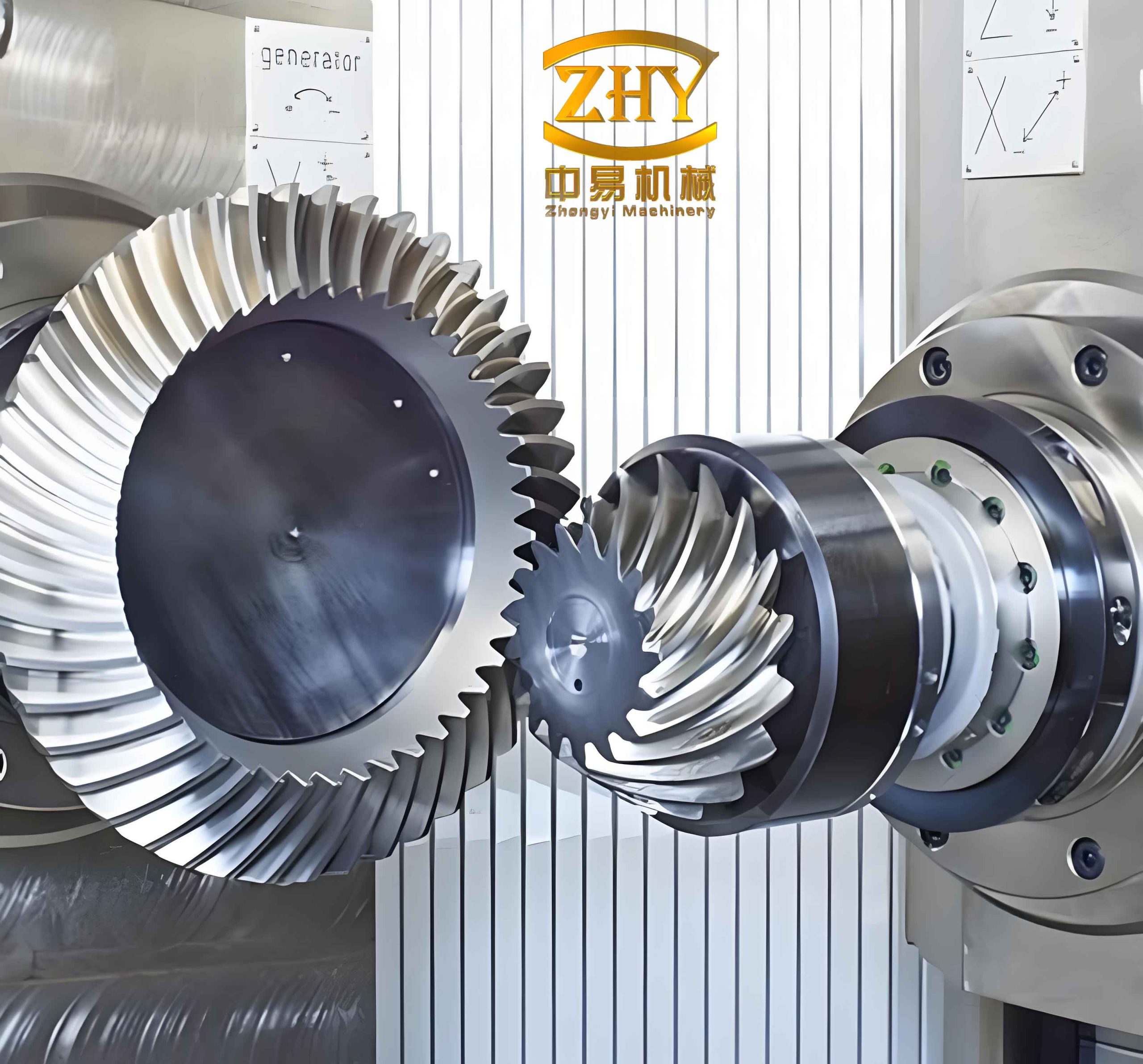
The design and manufacture of hyperboloidal gears, commonly known as hypoid gears, represent one of the most complex challenges in gear engineering. Their superior torque transmission capability and ability to accommodate non-intersecting, offset axes make them indispensable in automotive drivetrains, particularly in rear axles. Central to their performance is the tooth contact pattern—the elliptical region on the tooth flank where power is actually transmitted during meshing. The size, location, and shape of this contact pattern directly dictate the gear set’s load-carrying capacity, fatigue life, endurance strength, and noise-vibration-harshness (NVH) characteristics. Historically, the evaluation and optimization of this contact have heavily relied on the skill of experienced technicians using bench testing methods like marking compounds. This article presents, from my engineering perspective, a novel, comprehensive analysis system that transitions this process from an art to a rigorous science. This system establishes a direct digital thread from fundamental geometric theory through machine tool settings to the simulation and analysis of both theoretical and manufactured tooth flanks under load.
1. Fundamental Meshing Theory and Pitch Cone Relationships
The entire geometric foundation of a hyperboloidal gears pair can be derived from the spatial relationship between their pitch cones. Unlike bevel gears, the axes of hyperboloidal gears do not intersect, introducing a crucial offset dimension $E$. The pitch cones are conceptual surfaces that roll without sliding on each other, defining the kinematical basis for the gear pair.
Consider a pinion and a gear with their respective pitch cones. Each cone is defined by three fundamental parameters: the pitch cone angle ($\delta$), the pitch cone distance or apex distance ($A$), and the spiral angle ($\psi$). The relative positioning of these cones is governed by the assembly parameters: the shaft angle ($\Sigma$), the offset ($E$), and the mounting distances for the pinion ($J_P$) and gear ($J_G$). The following six fundamental equations interrelate these twelve key parameters (six per member), forming the cornerstone for all subsequent design and analysis of hyperboloidal gears:
$$ \cos\Sigma = -\sin\delta_P \sin\delta_G + \cos\delta_P \cos\delta_G \cos(\psi_P + \psi_G) $$
$$ E = \frac{(A_P \tan\delta_P + A_G \tan\delta_G) \cdot \cos\delta_P \cos\delta_G \sin(\psi_P + \psi_G)}{\sin\Sigma} $$
$$ \sin\eta = \frac{\cos\delta_P}{\sin\Sigma} \sin(\psi_P + \psi_G) $$
$$ \sin\xi = \frac{\cos\delta_G}{\sin\Sigma} \sin(\psi_P + \psi_G) $$
$$ J_P = \frac{E / \tan\eta}{\sin\Sigma} – A_P \sin\delta_P \tan\delta_P $$
$$ J_G = \frac{E / \tan\xi}{\sin\Sigma} – A_G \sin\delta_G \tan\delta_G $$
Given a target set of assembly parameters ($\Sigma$, $E$, $J_P$, $J_G$) and desired spiral angles, these equations can be solved to determine the required pitch cone geometries ($A_P$, $\delta_P$, $A_G$, $\delta_G$). Conversely, starting from defined pitch cones, the assembly dimensions can be calculated. This bidirectional relationship is pivotal. The following table summarizes the core parameters involved:
| Parameter | Symbol | Description |
|---|---|---|
| Shaft Angle | $\Sigma$ | Angle between the pinion and gear axes. |
| Offset | $E$ | Perpendicular distance between the axes of the hyperboloidal gears. |
| Pitch Cone Angle | $\delta_{P}, \delta_{G}$ | Angle between the gear axis and the pitch cone element. |
| Pitch Cone Distance | $A_{P}, A_{G}$ | Distance from the pitch cone apex to the gear back face. |
| Spiral Angle | $\psi_{P}, \psi_{G}$ | Angle of the tooth trace relative to the pitch cone element at the mean point. |
| Mounting Distance | $J_{P}, J_{G}$ | Axial distance from a reference datum to the gear back face during assembly. |
2. Determination of Machine Tool Settings
The transformation from theoretical geometry to a physical tooth flank is achieved through the precise setup of the gear cutting machine. For hyperboloidal gears, this typically involves a face-milling or face-hobbing process using a cutter head. The core principle is that the relative motion between the imaginary generating gear (represented by the cutter head) and the workpiece (the gear blank) must replicate the intended meshing condition.
2.1 Gear (Ring Gear) Machine Settings
The gear is generally cut using the Formate or Spread Blade method, where the cutter head’s blades generate the tooth slots directly. The machine settings position the gear blank relative to the rotating cutter head to simulate its conjugate action with an imaginary pinion. The primary settings include the machine root angle, the sliding base setting (to control tooth depth), the radial distance, and the angular position of the cradle. These are more straightforward to determine as they directly correspond to the gear’s own pitch cone geometry and blank data.
2.2 Pinion Machine Settings: The Heart of Contact Pattern Control
Pinion cutting is significantly more complex and is the primary means for tailoring the contact pattern of hyperboloidal gears. The pinion is cut using a generating process (Single Cycle or Completing Cycle), where the cutter head and the pinion blank undergo a prescribed rolling motion, simulating the pinion’s mesh with its mating gear. The key insight is that during pinion cutting, the machine settings are derived by considering the spatial relationship between the pinion’s pitch cone and the pitch cone of its imaginary mating gear. This imaginary gear’s parameters are initially based on the physical gear’s geometry but are deliberately altered through a series of “machine setting corrections” to pre-correct the tooth flank and achieve the desired loaded contact pattern.
These corrections, often termed as “ease-off” modifications, include:
- Modified Roll ($$Delta R$$): A slight deviation from the theoretical rolling ratio during generation, which primarily controls the lengthwise curvature of the pinion flank, affecting the contact pattern’s length and bias.
- Cutter Radius Change ($$Delta r_c$$): Adjusts the nominal radius of the cutter head, influencing the profile curvature of the pinion tooth.
- Cradle Angle Tilt ($$Delta i$$): Alters the basic machine root angle for the pinion, impacting the pressure angle and root clearance.
- Sliding Base ($$Delta X_B$$) and Radial Setting ($$Delta S_R$$): Fine-tune the depth and position of the cut.
The selection and combination of these parameters are the essence of the gear designer’s skill, now systematized through the proposed analysis framework. The table below categorizes common machine setting adjustments for hyperboloidal gears:
| Adjustment Parameter | Symbol | Primary Effect on Pinion Flank & Contact Pattern |
|---|---|---|
| Modified Roll | $\Delta R$ | Changes lengthwise curvature. Controls contact pattern length, toe-heel bias, and sensitivity to misalignment. |
| Cutter Radius Change | $\Delta r_c$ | Changes profile (transverse) curvature. Controls contact pattern width and pressure angle. |
| Cradle Angle Tilt | $\Delta i$ | Alters the basic pressure angle. Affects root clearance and contact pattern height on the tooth. |
| Sliding Base | $\Delta X_B$ | Adjusts the depth of cut. Fine-tunes the contact pattern position along the face width. |
| Radial Setting | $\Delta S_R$ | Adjusts the distance from the cutter center to the gear axis. Affects tooth thickness and contact centralization. |
3. Three-Dimensional Tooth Flank Modeling via Coordinate Transformation
The cornerstone of the new analysis system is a robust mathematical model for the tooth flank surface. For hyperboloidal gears, this is not a simple standard surface but a complex envelope generated by the motion of the cutter blades. The modeling process employs a chain of homogeneous coordinate transformations to track a point on the cutting edge from the cutter coordinate system to the finished gear coordinate system.
The fundamental transformation sequence is as follows:
- Cutter Blade Edge Definition: A point $P_c$ on the straight or profile-relieved cutting edge is defined in the Cutter Blade Coordinate System $(O_c – x_c y_c z_c)$.
- Transformation to Cutter Head: $P_c$ is transformed to the Cutter Head Coordinate System $(O_h – x_h y_h z_h)$ by applying rotations corresponding to the blade’s angular position.
- Transformation to Machine Cradle: The point is then transformed to the Cradle Coordinate System $(O_q – x_q y_q z_q)$, which incorporates the cutter head’s radial setting $S_R$, initial cradle angle $q_0$, and its rotational motion $\phi_c$ (for generating motions).
- Transformation to Gear Blank: Finally, the point is transformed into the stationary Gear Blank Coordinate System $(O_g – x_g y_g z_g)$ through transformations involving the machine root angle $\gamma_m$, sliding base $X_B$, and the work rotation $\phi_w$ which is kinematically linked to the cradle rotation via the ratio of generation $R_g$ ($\phi_w = \phi_c / R_g$).
The overall transformation can be expressed as:
$$ P_g = \mathbf{T}_{g \leftarrow q} \cdot \mathbf{T}_{q \leftarrow h} \cdot \mathbf{T}_{h \leftarrow c} \cdot P_c $$
where $\mathbf{T}_{i \leftarrow j}$ are the 4×4 homogeneous transformation matrices.
By calculating the trajectory of multiple points along the cutting edge through a series of cradle/work positions, a dense point cloud representing the entire active tooth flank of the hyperboloidal gears is generated. Surface fitting techniques are then applied to create a continuous digital twin of the flank, complete with root, tip, heel, and toe boundaries. This model is valid for both the theoretical design flank and can be adapted to represent actual measured flanks from a Coordinate Measuring Machine (CMM) by using the measured point cloud as the starting data.
4. Loaded Tooth Contact Analysis (LTCA) Methodology
The ultimate goal is to predict the contact pattern under realistic operating conditions. The system performs a quasi-static Loaded Tooth Contact Analysis directly on the 3D flank models. This method supersedes traditional unloaded kinematic TCA by accounting for tooth bending and contact deformations.
4.1 The Core Algorithm: Minimum Distance Scanning
The analysis simulates the meshing cycle as one gear rotates incrementally relative to the other. For each discrete angular position $\theta$, the following steps are executed:
- Positioning: The digital models of the pinion and gear flanks are positioned according to the nominal assembly settings ($\Sigma$, $E$, $J_P$, $J_G$) and the current rotation angle.
- Proximity Search: For a grid of points on the pinion flank, the system calculates the shortest distance (along the common surface normal direction) to the opposing gear flank. This distance, when subtracted from the nominal backlash, represents the potential penetration or separation.
- Compliance and Load Distribution: The potential penetrations are treated as initial overlaps. A global compliance matrix is constructed, incorporating:
- Local Contact Compliance: Based on Hertzian contact theory for elastic bodies. The contact stiffness for a point pair is a function of local curvatures and material properties (Young’s modulus $E$, Poisson’s ratio $\nu$). For two cylinders in contact, the half-width $b$ is:
$$ b = \sqrt{\frac{4 F}{\pi L} \frac{\frac{1-\nu_1^2}{E_1} + \frac{1-\nu_2^2}{E_2}}{\frac{1}{R_1} + \frac{1}{R_2}}} $$
where $F$ is load per unit length $L$, and $R$ are principal radii of curvature. - Tooth Bending and Shear Compliance: Calculated using cantilever beam models or, more accurately, Finite Element Method (FEM) substructuring.
- Gear Body Deflection: Often derived from prior full-gear FEM analyses.
- Local Contact Compliance: Based on Hertzian contact theory for elastic bodies. The contact stiffness for a point pair is a function of local curvatures and material properties (Young’s modulus $E$, Poisson’s ratio $\nu$). For two cylinders in contact, the half-width $b$ is:
- Solving the System: The equilibrium equation $\mathbf{K} \cdot \mathbf{\delta} = \mathbf{F}$ is solved, where $\mathbf{K}$ is the global stiffness matrix, $\mathbf{\delta}$ is the vector of total deformations (including initial separations), and $\mathbf{F}$ is the vector of unknown contact forces. This yields the final loaded contact pressures and the deformed state of the hyperboloidal gears.
- Contact Pattern Visualization: For each meshing position, the areas where the contact pressure exceeds a threshold (e.g., >0) are projected onto the tooth flank. The cumulative result across all positions defines the dynamic contact pattern. The path of the contact ellipse’s center defines the contact trace.
4.2 Integration with Manufacturing and Validation
The power of this system lies in its seamless integration throughout the product lifecycle. After each major manufacturing step—rough cutting, heat treatment, grinding/lapping—the physical gear can be measured on a CMM. The resulting point cloud data is imported directly into the analysis system, replacing the theoretical flank model.
The analysis is then run on this “as-manufactured” geometry. This allows for:
- Predictive Quality Assurance: Forecasting the contact pattern and transmission error before the gear is ever assembled in a housing or run on a tester.
- Root Cause Analysis: If bench-test results deviate from predictions, the measured flanks of both mating hyperboloidal gears can be analyzed to determine whether the deviation stems from cutting errors, heat treatment distortion, or assembly misalignment.
- Process Optimization: Correlating specific machine setting adjustments with their quantified effects on the loaded contact pattern, thereby building a knowledge base for future designs.
The workflow from design to validation is summarized below:
| Stage | Input Data | System Action | Output/Purpose |
|---|---|---|---|
| Design | Macro-geometry, Target Contact Pattern | Calculate theoretical machine settings. Perform LTCA on theoretical flanks. | Optimize settings for desired performance (load capacity, noise). |
| Post-Cutting | CMM data from cut gears | Run LTCA on as-cut flank geometry. | Verify cutting process; predict contact before heat treat. |
| Post-Grinding | CMM data from finished gears | Run final LTCA on finished geometry. | Final performance prediction and quality certification. |
| Troubleshooting | CMM data from problematic gears; bench test results | Compare LTCA results with bench test. Identify flank geometry deviations causing poor contact. | Root cause identification for corrective action. |
5. Conclusion and Performance Outcomes
The development and implementation of this integrated analysis system for hyperboloidal gears marks a significant advancement. By establishing a rigorous mathematical foundation based on pitch cone relationships, enabling precise 3D flank modeling via coordinate transformations, and executing a sophisticated loaded tooth contact analysis, the system creates a closed-loop digital process. It bridges the gap between design intent, manufacturing execution, and performance validation. The system’s ability to handle both theoretical and measured data from any stage of production is particularly powerful.
When applied to develop high-torque hyperboloidal gears for next-generation automotive transmissions, this methodology yields concrete benefits. Engineers can now proactively optimize the contact pattern to achieve two often-conflicting goals simultaneously: maximizing surface durability and bending strength for high endurance, while minimizing transmission error and its associated gear whine for superior NVH performance. The result is a more robust, quieter, and more reliable gear set, achieved through a deterministic engineering process rather than trial and error. This systematic approach ultimately reduces development time, improves first-time quality, and pushes the performance boundaries of these critical mechanical components.