
In the realm of power transmission, hypoid bevel gears hold a position of critical importance, especially in applications demanding compact design, high torque capacity, and smooth operation at non-intersecting axes. Their unique geometry, characterized by offset axes, allows for lower positioning of driveshafts in automotive rear axles, contributing to improved vehicle stability and cabin space. However, this very complexity makes the mechanical analysis of hypoid bevel gears profoundly challenging. Predicting performance parameters like contact stress, root bending stress, and transmission error under dynamic loading conditions is essential for ensuring durability, reducing noise, and preventing catastrophic failure.
Traditional analytical methods, while valuable, often rely on significant simplifications and require deep mathematical expertise for implementing algorithms like Tooth Contact Analysis (TCA). The advent of powerful finite element analysis (FEA) software has revolutionized this field. Among these tools, ANSYS/LS-DYNA stands out for performing explicit dynamic analysis, making it exceptionally well-suited for simulating transient events like impact, severe deformation, and complex surface-to-surface contact—all of which are inherent to the meshing process of hypoid bevel gears. This article details a first-person perspective on the methodology for conducting a high-fidelity dynamic contact simulation of a hypoid gear pair, from model creation to post-processing of results, leveraging the capabilities of ANSYS/LS-DYNA.
Theoretical Background and Simulation Rationale
The core challenge in analyzing hypoid bevel gears lies in their spatially curved, conjugate tooth surfaces. The contact between two such surfaces is not a simple line or point but a complex elliptical patch that moves across the tooth flank during meshing. The pressure distribution within this patch is highly non-uniform and transient. Classical Hertzian contact theory provides a foundational understanding but is limited to simple geometries and static conditions. For dynamic, multi-tooth engagement scenarios, a numerical approach is indispensable.
Explicit dynamics, as implemented in LS-DYNA, solves the equations of motion using a central difference time integration scheme. It is conditionally stable, with the time step limited by the smallest element size in the model (Courant condition). This method is highly efficient for short-duration, dynamic events where inertial forces are significant. The contact algorithm in LS-DYNA enforces constraints to prevent penetration and calculates interface forces based on a penalty method, optionally including friction. This makes it ideal for simulating the successive engagement and disengagement of gear teeth, capturing the shock-like loading at the beginning of contact and the load sharing between multiple pairs of hypoid bevel gears.
The fundamental equations governing the motion are:
$$ \mathbf{M}\ddot{\mathbf{u}}_t + \mathbf{C}\dot{\mathbf{u}}_t + \mathbf{K}\mathbf{u}_t = \mathbf{F}_t^{\text{ext}} $$
where $\mathbf{M}$ is the mass matrix, $\mathbf{C}$ is the damping matrix, $\mathbf{K}$ is the stiffness matrix, $\ddot{\mathbf{u}}_t$, $\dot{\mathbf{u}}_t$, and $\mathbf{u}_t$ are the nodal acceleration, velocity, and displacement vectors at time $t$, and $\mathbf{F}_t^{\text{ext}}$ is the external force vector including contact forces. The explicit scheme solves for acceleration at time $t$ and then integrates to find velocity and displacement at time $t+\Delta t$.
The contact force for a slave node penetrating a master segment is calculated as:
$$ \mathbf{f}_c = k_c \cdot d \cdot \mathbf{n} + \text{friction component} $$
where $k_c$ is the penalty stiffness, $d$ is the penetration depth, and $\mathbf{n}$ is the normal vector to the master segment. For elastic materials, an approximate Hertzian-like pressure $p_0$ over an elliptical contact area with semi-axes $a$ and $b$ can be conceptually related to the FEA results:
$$ p_0 = \frac{3F}{2\pi a b} $$
$$ a = \alpha \sqrt[3]{\frac{3F R’}{4E’}}, \quad b = \beta \sqrt[3]{\frac{3F R’}{4E’}} $$
$$ \frac{1}{E’} = \frac{1-\nu_1^2}{E_1} + \frac{1-\nu_2^2}{E_2}, \quad \frac{1}{R’} = \frac{1}{R_{1}} + \frac{1}{R_{2}} $$
Here, $F$ is the total contact force, $E’$ is the equivalent Young’s modulus, $R’$ is the equivalent relative curvature, and $\alpha$, $\beta$ are coefficients dependent on the ellipticity of the contact. The simulation computes this interaction dynamically for every time step.
Simulation Workflow: A Step-by-Step Account
1. Geometry Modeling and Import
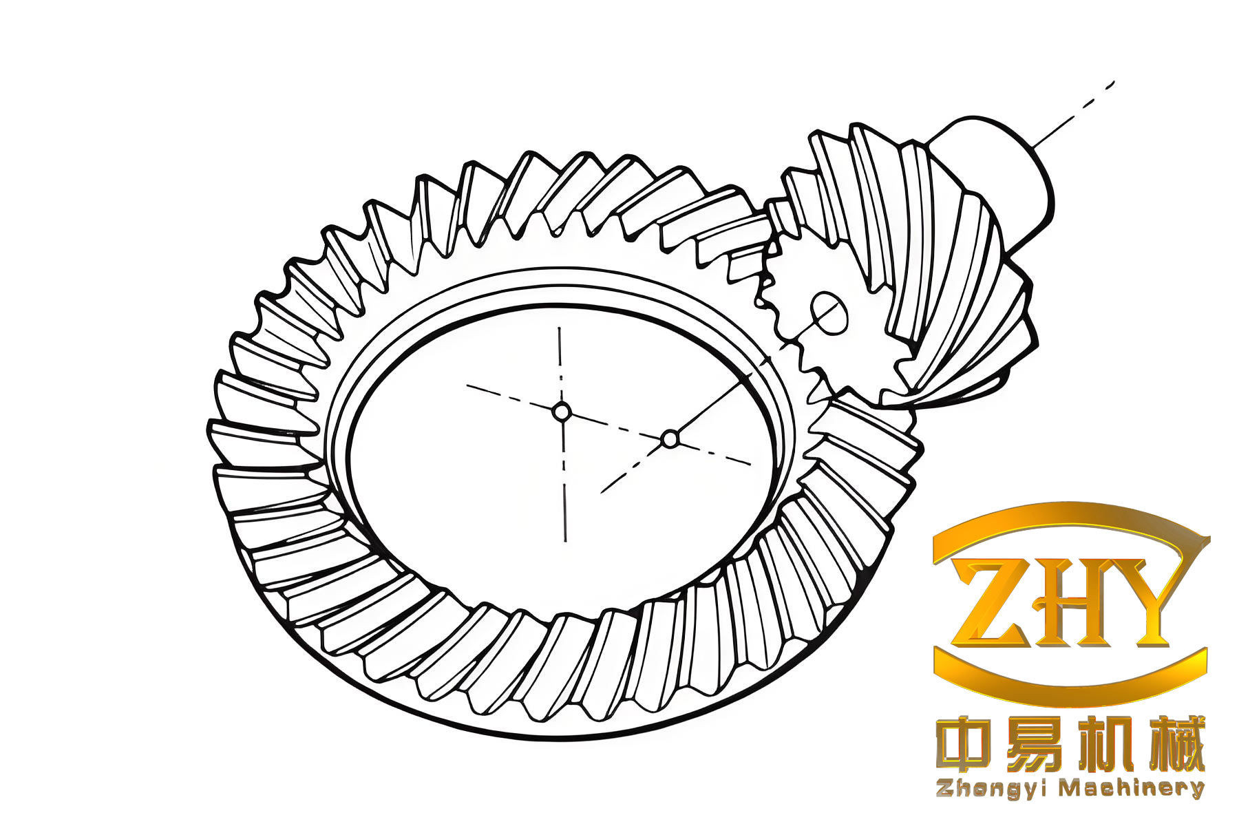
The journey begins with an accurate 3D geometric model. The complex tooth geometry of hypoid bevel gears is defined by sophisticated machine tool settings and requires generation via specialized gear design software or mathematical programming. In this case, the tooth surface points were generated by solving the meshing equations using MATLAB. This point cloud data defines the active tooth flanks. The solid model was then constructed in a CAD environment using these surfaces and imported into ANSYS. The following figure illustrates the intricate geometry of a hypoid bevel gear pair, highlighting the offset between the axes and the curved tooth profiles.
2. Preprocessing in ANSYS
This phase involves preparing the geometry for the solver. It is the most crucial step for ensuring an accurate and stable simulation.
a. Element Type Selection
Two key element types are selected:
- SOLID164: An 8-node hexahedral element used for the 3D discretization of the gear teeth. It is well-suited for large deformation and contact problems.
- SHELL163: A 4-node quadrilateral shell element. A critical step involves defining a layer of SHELL163 elements on the inner bore surfaces of both the pinion and gear. These shell elements are then assigned rigid body properties. Since SOLID164 lacks rotational degrees of freedom, applying torque directly to a solid part is non-trivial. By coupling the motion of the solid gear teeth to a rigid body defined by shells, we can easily prescribe angular velocity and torque about its center of mass. This approach dramatically reduces computational cost as the rigid body has only six degrees of freedom regardless of the number of nodes associated with it.
b. Material Properties
A common gear steel is used. Its properties are defined for the solid elements. The shell elements, being rigid, require only density and constraints.
| Property | Value | Unit |
|---|---|---|
| Density (ρ) | 7830 | kg/m³ |
| Young’s Modulus (E) | 2.07e11 | Pa |
| Poisson’s Ratio (ν) | 0.3 | – |
| Yield Strength | ~6.0e8 | Pa (Assumed) |
c. Meshing
The gears are meshed using a swept volume method. Special attention is paid to the contact regions on the tooth flanks. A finer mesh is necessary there to capture the high stress gradients accurately. The transition from fine mesh in contact zones to a coarser mesh in the core and rim is managed to optimize the number of elements. The final meshed assembly, showing the solid gear teeth and the inner shell “rigid” layers, is a critical checkpoint.
d. Defining Contact
The interaction between the pinion and gear teeth is modeled using a Surface-to-Surface (STS) contact algorithm. One gear’s tooth surfaces are defined as the “contact” surface, and the other’s as the “target” surface. A static and dynamic friction coefficient (e.g., 0.1) is defined. The penalty stiffness scale factor is often left at its default value initially but may require adjustment if excessive penetration is observed.
e. Applying Loads and Boundary Conditions
Local coordinate systems are created at the theoretical rotation centers (apex) of each gear. Loads are applied with reference to these local systems to ensure correct rotation axes.
- Driver (Pinion): A prescribed angular velocity (ω₁) and a driving torque (T₁) are applied to its rigid body (SHELL163 part).
- Driven (Gear): A prescribed (or initially zero) angular velocity and a resisting torque (T₂) are applied to its rigid body. The resisting torque simulates the load from the driveline.
The values are typically defined using array parameters over time. For a simple steady-state analysis, they are held constant after a brief ramp-up.
| Parameter | Pinion | Gear | Calculation Basis |
|---|---|---|---|
| Angular Velocity, ω | 628 rad/s (≈6000 RPM) | 141.3 rad/s | Gear Ratio |
| Input Torque, T_in | 1000 Nm | – | Given Power/Speed |
| Resisting Torque, T_resist | – | ~ (T_in * Ratio) Nm | Equilibrium (ideal) |
Constraints are applied to the rigid bodies to allow only rotation about their designated axes, suppressing all translational and other rotational degrees of freedom.
3. Solution Setup and Execution in LS-DYNA
Key solution parameters are set:
- Termination Time: Calculated to cover at least two to three mesh cycles for hypoid bevel gears. For a pinion speed of 6000 RPM (100 rev/s), one mesh cycle might be ~0.01s. A time of 0.002-0.005s is often sufficient to capture detailed contact events.
- Output Controls: The database (D3PLOT) output interval is set to capture enough frames for a smooth animation and for post-processing stress histories (e.g., every 1e-6s). Time-history (D3THDT) output is defined for specific nodes/elements to monitor force, stress, or displacement over time.
- Mass Scaling: To improve the computational efficiency, a carefully controlled mass scaling can be applied to increase the minimum stable time step, without significantly affecting the inertia-dominated dynamics.
- Hourglass Control: For under-integrated elements like SOLID164, hourglass control (e.g., Flanagan-Belytschko stiffness form) is activated to prevent spurious zero-energy deformation modes.
The model is then exported as a LS-DYNA keyword file (.k). If the model is large, memory allocation in the .k file header is increased. The simulation is run using the LS-DYNA solver.
Results, Discussion, and Engineering Insights
Post-processing in LS-PrePost or ANSYS post-processors reveals the dynamic behavior of the hypoid bevel gears in exceptional detail.
Contact Stress Evolution
The simulation vividly shows the birth, movement, and extinction of the contact ellipses along the tooth flank path. The maximum contact (Hertzian) stress is not constant. It peaks when contact initiates near the tooth root or tip (due to higher curvature and potential edge contact) and varies as the contact patch moves through the central, more favorable region of the tooth. The explicit dynamics capture the slight impact at initial contact, visible as a high-frequency oscillation in the contact force trace before it stabilizes. The stress distribution within the elliptical patch is no longer perfectly elliptical as in classic Hertz theory but is modified by the edge geometry and neighboring material.
The equivalent (von Mises) stress shows the development of a subsurface stress maximum, which is critical for predicting pitting fatigue failure common in hypoid bevel gears. The location of this maximum von Mises stress, typically at a depth of 0.2-0.5 times the contact half-width, can be precisely identified.
Load Sharing Between Multiple Teeth
A significant advantage of simulating a multi-tooth segment (e.g., 3-5 teeth per gear) is the ability to study load sharing. The results clearly illustrate the transition of load from one pair of teeth to the next. There is a period of double-tooth contact where the total torque is shared between two pairs. The percentage of load carried by each pair during this phase is not necessarily 50/50; it depends on the relative stiffness and contact geometry of the two pairs at that specific instant. This transient load sharing behavior, difficult to assess analytically, is crucial for accurate root bending stress calculation and fatigue life prediction of hypoid bevel gears.
| Parameter | Pinion Tooth (Driving) | Gear Tooth (Driven) | Notes |
|---|---|---|---|
| Max. Contact Pressure | 1.45 GPa | 1.45 GPa | Peak occurs at initial contact |
| Contact Ellipse Semi-Major Axis | ~1.8 mm | ~1.8 mm | Varies along path of contact |
| Subsurface von Mises Max | 0.85 GPa (at ~0.3mm depth) | 0.85 GPa (at ~0.3mm depth) | Critical for pitting initiation |
| Root Bending Stress (Max) | 320 MPa | 280 MPa | Occurs at the highest single-tooth load point |
| Transmission Error (Peak-to-Peak) | ~0.8 micron | Calculated from angular displacement difference | |
Dynamic Effects and Implications
The explicit dynamic analysis captures effects often neglected in static analyses:
- Inertial Forces: At high rotational speeds, centrifugal forces can slightly alter the contact pattern and stress state.
- Stress Wave Propagation: The high-frequency content from impact loading can cause local stress concentrations.
- System Response: If the supporting shafts and bearings were included in the model (as flexible bodies), the simulation could predict system-level vibrations and noise, known as gear whine, which is a major concern for hypoid bevel gears in automotive applications.
These insights are invaluable for optimizing gear macro-geometry (pressure angle, spiral angle) and micro-geometry (modifications like tip relief, root relief, and crowning) to minimize transmission error, reduce contact stress peaks, and ensure smooth load transfer.
Engineering Applications and Concluding Remarks
The methodology outlined provides a powerful virtual prototyping tool for the design and analysis of hypoid bevel gears. It allows engineers to:
- Validate and Optimize Design: Before cutting physical prototypes, the contact pattern, pressure distribution, and bending stresses can be evaluated and optimized by adjusting machine tool settings.
- Predict Fatigue Life: The calculated time histories of contact and bending stress serve as direct input for fatigue life prediction models (e.g., using the Ioannides-Harris or Lundberg-Palmgren equations for rolling contact fatigue).
- Investigate Failure Modes: The simulation can help diagnose root causes of failures like pitting, spalling, or tooth breakage by visualizing the stress conditions that lead to them.
- Assess Manufacturing Errors: The effect of misalignments (offset error, shaft angle error) or tooth surface deviations on load distribution and stress can be studied by intentionally introducing these variations into the model.
In conclusion, leveraging ANSYS/LS-DYNA for the dynamic contact simulation of hypoid bevel gears bridges the gap between complex theoretical gear geometry and practical engineering performance assessment. It transforms the design process from one reliant on experience and iterative physical testing to a predictive, simulation-driven endeavor. While computationally demanding, the depth of insight gained into the transient meshing mechanics, load sharing, and stress evolution is unparalleled, enabling the development of more robust, efficient, and quieter gear drives for the most demanding applications. Future advancements will integrate this approach with system-level multi-body dynamics and advanced material models to further close the loop between digital design and real-world performance.