
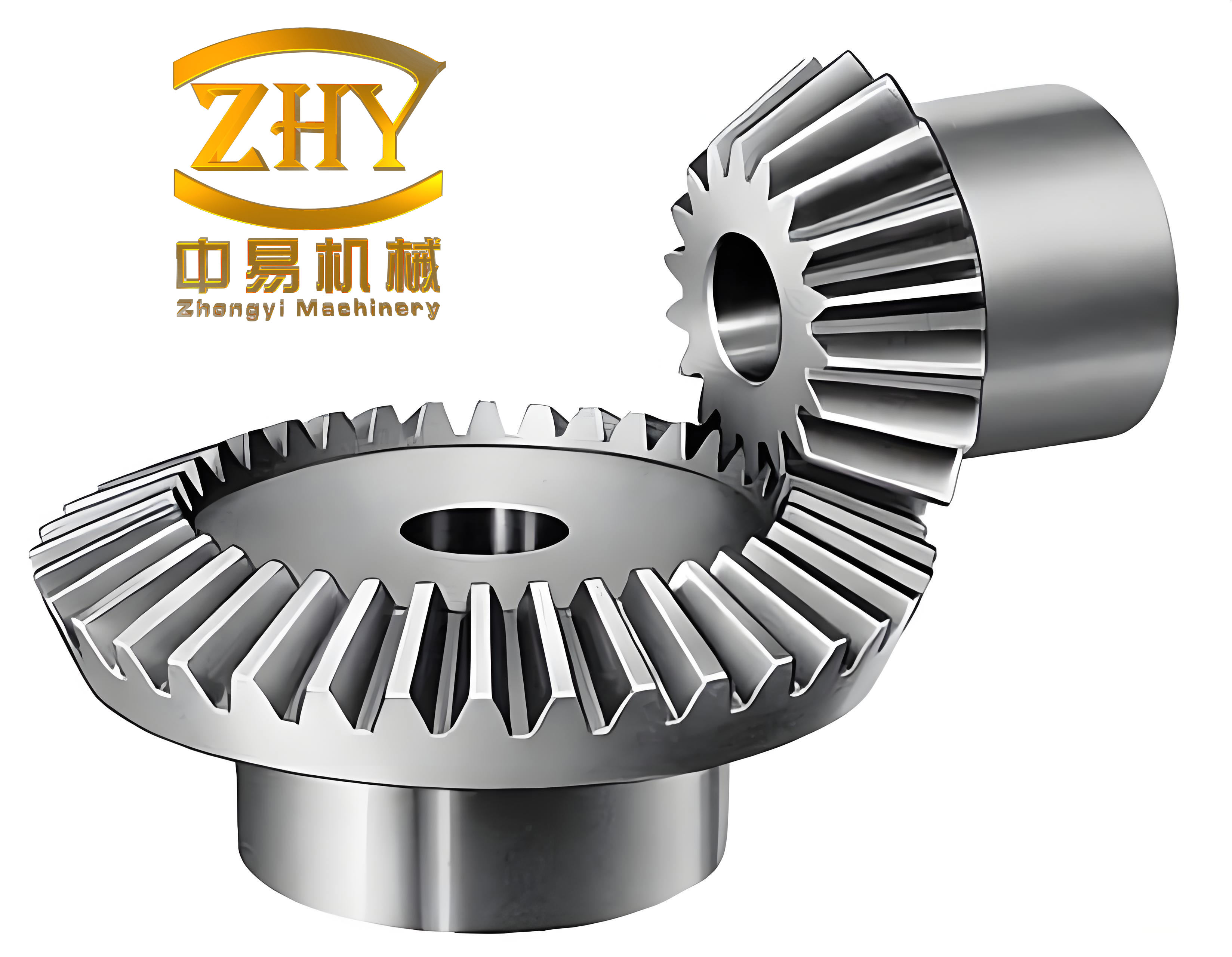
In my extensive experience working with gear manufacturing, particularly for straight bevel gears, I have often encountered situations where high-precision grinding equipment is unavailable, especially in small to medium-sized workshops. When the required machining accuracy for straight bevel gears is not exceptionally high, a practical and accessible solution is needed. I have found that the tooth profile for a disk-type milling cutter used to machine these straight bevel gears can be efficiently determined using a graphical method. This approach is not only simple in its drafting steps but also greatly facilitates the manufacture of the cutter’s tooth profile template. The core advantage lies in its independence from sophisticated curve grinding machines, making it a valuable technique for many practical applications involving straight bevel gears.
The fundamental principle, or the “rationale” behind this graphical method, is rooted in the concept of the equivalent spur gear. The tooth profile of the milling cutter must correspond to the tooth space of the straight bevel gear. However, due to the tapered geometry of a straight bevel gear, the tooth profile varies from the large end to the small end. The established theory states that the tooth profile of the disk-type milling cutter should be based on the tooth form of the equivalent spur gear at the large end of the straight bevel gear, while its width is determined by the tooth space width at the small end’s equivalent gear.
Consider the machining process. When the cutter engages the gear blank, it can only generate the tooth profile at a specific point, say point $$A$$ on the large end. To machine the entire tooth flank of the straight bevel gear, either the gear blank must be rotated by a certain angle $$\lambda$$, or equivalently, the cutter’s axis must be tilted by the complementary angle. This relative motion ensures that the cutter’s tooth profile correctly envelopes the desired gear tooth. Therefore, if we design the cutter’s tooth profile as the mirror image of the large-end equivalent gear’s tooth form, and position it symmetrically about an axis that accounts for this relative tilt, the resulting cutter will successfully machine the straight bevel gear. This forms the cornerstone of our graphical construction method for the straight bevel gear milling cutter.
Let me now detail the step-by-step graphical procedure I routinely follow. The entire process hinges on accurately constructing the approximate tooth form of the large-end equivalent spur gear using circular arcs—a technique often referred to as the “circular-arc approximation method” for the involute curve.
Step 1: Determine the Equivalent Gear Parameters.
First, calculate the virtual number of teeth $$z_v$$ for the large-end equivalent spur gear of the straight bevel gear. The formula is:
$$z_v = \frac{z}{\cos \delta}$$
where $$z$$ is the actual number of teeth of the straight bevel gear and $$\delta$$ is its pitch cone angle. Based on $$z_v$$, select the appropriate cutter number from standard indexing tables. The module $$m$$ for this calculation is the module of the straight bevel gear at its large end.
Step 2: Calculate Key Radii and Draw Base Circles.
Compute the four critical radii for the large-end equivalent gear:
– Addendum circle radius: $$r_a = m \left( \frac{z_v}{2} + 1 \right)$$
– Pitch circle radius: $$r = m \cdot \frac{z_v}{2}$$
– Base circle radius: $$r_b = r \cos \alpha$$, where $$\alpha$$ is the cutter pressure angle (typically 20° or 14.5°).
– Dedendum circle radius: $$r_f = m \left( \frac{z_v}{2} – 1.25 \right)$$
Draw these concentric circles on the drafting sheet, with their common center at point $$O$$.
Step 3: Establish the Reference Point.
On the pitch circle, locate point $$P$$ such that the arc length from the vertical axis to $$P$$ is equal to one-quarter of the circular pitch. Mathematically, the angle subtended is:
$$\theta = \frac{\pi m}{4r} = \frac{\pi}{2z_v} \text{ radians}$$
This point $$P$$ is crucial for initiating the tooth profile construction.
Step 4: Construct the Tooth Profile Using Circular Arcs.
The involute profile is approximated by two (or sometimes three) tangential circular arcs. The radii and centers for these arcs are determined using coefficients tabulated for specific pressure angles. The procedure bifurcates based on the relationship between the base circle radius $$r_b$$ and the dedendum circle radius $$r_f$$.
Case A: When $$r_b > r_f$$ (which is common for gears with higher tooth counts).
– The tooth profile from the addendum down to the base circle is approximated by a circular arc. Its center $$O_1$$ lies on the line connecting the gear center $$O$$ and point $$P$$. The radius $$R_1$$ is given by $$R_1 = K_1 \cdot m$$, where $$K_1$$ is a coefficient from the table.
– Draw this arc from point $$P$$ upwards to the addendum circle and extend it slightly to point $$A$$. This forms the top segment of the tooth profile.
– The tooth profile from the base circle down to the dedendum circle is approximated by another circular arc. Its center $$O_2$$ is also located on the line $$OP$$. The radius $$R_2$$ is given by $$R_2 = K_2 \cdot m$$, where $$K_2$$ is another coefficient.
– Draw this arc from a point on the base circle (determined by the geometry) down to the dedendum circle.
Case B: When $$r_b \leq r_f$$ (common for gears with low tooth counts).
In this case, the profile below the base circle is often a straight line or a simple arc connecting to the root fillet. The specific construction uses different coefficients and sometimes a straight radial line from the base circle to the root circle, blended with a fillet arc. The coefficients for the fillet radius $$R_f$$ are also tabulated.
The values for the coefficients $$K_1$$, $$K_2$$, and the locations of centers $$O_1$$ and $$O_2$$ (defined by distances $$L_1$$ and $$L_2$$ from gear center $$O$$) are pre-calculated for standard pressure angles. They are universally applicable once the virtual number of teeth $$z_v$$ is known. Below, I provide these essential coefficient tables. Note that for actual calculation, the coefficient values must be multiplied by the module $$m$$ of the straight bevel gear.
| Cutter Number | Virtual Teeth Range $$z_v$$ | $$K_1$$ | $$L_1/m$$ | $$K_2$$ | $$L_2/m$$ | Fillet Radius Coeff. $$K_f$$ | Angle $$\beta$$ (deg) |
|---|---|---|---|---|---|---|---|
| 1 | 12-13 | 1.218 | 0.342 | 0.735 | 0.668 | 0.25 | 30 |
| 2 | 14-16 | 1.191 | 0.355 | 0.758 | 0.653 | 0.25 | 29 |
| 3 | 17-20 | 1.168 | 0.367 | 0.778 | 0.640 | 0.25 | 28 |
| 4 | 21-25 | 1.148 | 0.378 | 0.796 | 0.628 | 0.25 | 27 |
| 5 | 26-34 | 1.131 | 0.388 | 0.812 | 0.618 | 0.25 | 26 |
| 6 | 35-54 | 1.115 | 0.397 | 0.827 | 0.609 | 0.25 | 25 |
| 7 | 55-134 | 1.101 | 0.406 | 0.840 | 0.601 | 0.25 | 24 |
| 8 | 135 & above | 1.088 | 0.414 | 0.852 | 0.594 | 0.25 | 23 |
| Cutter Number | Virtual Teeth Range $$z_v$$ | $$K_1$$ | $$L_1/m$$ | $$K_2$$ | $$L_2/m$$ | Fillet Radius Coeff. $$K_f$$ | Angle $$\beta$$ (deg) |
|---|---|---|---|---|---|---|---|
| 1 | 12-13 | 1.512 | 0.275 | 0.910 | 0.725 | 0.31 | 37 |
| 2 | 14-16 | 1.473 | 0.288 | 0.935 | 0.712 | 0.31 | 36 |
| 3 | 17-20 | 1.439 | 0.300 | 0.958 | 0.700 | 0.31 | 35 |
| 4 | 21-25 | 1.409 | 0.311 | 0.978 | 0.689 | 0.31 | 34 |
| 5 | 26-34 | 1.382 | 0.321 | 0.997 | 0.679 | 0.31 | 33 |
| 6 | 35-54 | 1.358 | 0.331 | 1.014 | 0.669 | 0.31 | 32 |
| 7 | 55-134 | 1.336 | 0.340 | 1.030 | 0.660 | 0.31 | 31 |
| 8 | 135 & above | 1.316 | 0.348 | 1.044 | 0.652 | 0.31 | 30 |
Step 5: Derive the Milling Cutter Tooth Profile.
The curve we have constructed (the approximate involute from addendum to dedendum) represents one side of the large-end equivalent gear tooth space. However, for the straight bevel gear milling cutter, we need the mirror image of this curve. The axis of symmetry for the cutter tooth profile is not the vertical axis of the gear drawing but is rotated by the angle $$\lambda$$ mentioned earlier. This angle $$\lambda$$ is determined by the geometry of the straight bevel gear and ensures the cutter will generate the correct tapered tooth form. Its calculation involves the pitch cone angle and the position along the tooth length. For practical graphical purposes, after constructing the gear tooth space profile, we draw the line representing the cutter’s axis of symmetry at the calculated angle $$\lambda$$ from the vertical. The complete cutter tooth profile is then obtained by taking the constructed curve and its mirror image across this new axis of symmetry. The width of the cutter tooth at the reference line is made equal to the space width at the small-end equivalent gear, which can be calculated as:
$$W_{small} = \frac{\pi m}{2} – 2m \left( \tan \alpha \right) \cdot \text{(correction factor for small end)}$$
Often, for simplicity and given the accuracy context, this width is taken directly from standard tooth thickness calculations applied to the small-end dimensions of the straight bevel gear.
Step 6: Address the Transition/Filter Curve.
The root of the gear tooth, and consequently the tip of the cutter tooth, usually includes a fillet to avoid stress concentration. The graphical method incorporates this. For cutter numbers 1 to 5 (typically), the tip of the cutter tooth profile often consists of a straight line segment tangent to a circular arc. The angle of this line and the radius of the arc are defined by the angle $$\beta$$ and the coefficient $$K_f$$ from the tables, where the fillet radius $$R_f = K_f \cdot m$$. For cutter numbers 6 to 8, the tip might be formed by a single circular arc blending smoothly with the main profile. The drawing must ensure tangential continuity between all segments—the main approximated involute arc(s) and the fillet arc or line.
To solidify understanding, let’s express some key relationships mathematically. The angle $$\lambda$$, though often determined from setting charts, can be approximated for a point on the pitch circle at the large end by considering the generation process. The relative rotation needed aligns the cutter axis with the tooth normal at that point. A functional approximation is:
$$\lambda \approx \frac{90^\circ}{z_v} + \text{arcsin}\left(\frac{m \sin\alpha}{r_b}\right)$$
This formula highlights the dependency on the virtual number of teeth $$z_v$$ of the straight bevel gear’s equivalent gear. The primary goal, however, is the graphical layout, and precise calculation of $$\lambda$$ can be sourced from specialized texts on straight bevel gear generation.
The entire graphical process I’ve described effectively translates the complex three-dimensional problem of straight bevel gear machining into a two-dimensional drafting exercise. Once the full cutter tooth profile is drawn, it can be used directly to manufacture a template for grinding or profiling the actual disk-type milling cutter. This method’s beauty is its visual clarity. One can see how changes in the straight bevel gear parameters—like the number of teeth $$z$$, the pitch cone angle $$\delta$$, or the module $$m$$—affect the shape of the cutter profile through the intermediate variable $$z_v$$ and the selected coefficients.
Let’s delve deeper into the advantages of this method, particularly for machining straight bevel gears. First, it democratizes the ability to produce custom or replacement cutters. Not every workshop has access to CNC gear grinding machines or sophisticated CAD/CAM software for generating precise involute curves. The graphical method requires only basic drafting tools, the provided coefficient tables, and an understanding of the underlying geometry of the straight bevel gear. Second, it is fast. For a one-off job or a small batch production of straight bevel gears, spending days on digital modeling and programming might be inefficient compared to a few hours of drafting. Third, the method inherently builds in an allowance for the approximation error. The circular-arc approximation to the true involute is extremely close for the intended range of machining accuracy (“when processing accuracy requirements are not high”). The errors introduced are well within acceptable limits for many applications, such as in agricultural machinery, certain automotive differentials, or material handling equipment where the straight bevel gear operates at moderate speeds and loads.
Furthermore, the technique encourages a deeper mechanistic understanding of the interaction between the cutter and the straight bevel gear workpiece. By manually plotting the profile, the engineer or machinist gains an intuitive feel for how the cutter’s shape directly imprints onto the gear’s tooth. This is invaluable for troubleshooting machining issues like undercutting or incorrect tooth contact patterns in straight bevel gears. One can visually assess whether the constructed profile has sufficient clearance at the root or if the tip is too pointed.
To illustrate the versatility, consider two distinct straight bevel gears: one with a small pitch cone angle (e.g., 15°) and many teeth, and another with a large pitch cone angle (e.g., 60°) and few teeth. For the first gear, the virtual number of teeth $$z_v$$ will be only slightly larger than $$z$$ (since $$\cos 15^\circ \approx 0.966$$). This will likely place it in a higher cutter number range (like #7 or #8), where the approximated profile uses arcs with larger radii, resulting in a very smooth, near-true involute form. For the second straight bevel gear, $$z_v$$ will be much larger (since $$\cos 60^\circ = 0.5$$, so $$z_v = 2z$$). This might also place it in a higher cutter number bracket, but the graphical construction proceeds identically. The resulting cutter will have a profile suited for a gear with a more pronounced taper. This consistent procedure handles the diversity of straight bevel gear geometries.
In practice, after obtaining the paper template from the drawing, it is transferred to a master gauge made of sheet metal. This gauge is then used to inspect the ground profile of the milling cutter blank. For manufacturing the cutter itself, a tool and cutter grinder can be set up using this gauge as a reference, perhaps with a pantograph attachment if available, to replicate the complex curve. Even without a pantograph, a skilled grinder can approximate the shape by “touching” the grinding wheel to various points guided by the template, achieving a serviceable cutter for the straight bevel gear.
It is also worth discussing the limitations. This graphical method is expressly for straight bevel gears with low to moderate precision requirements. For high-precision, high-speed, or high-load applications, such as in aerospace or precision gearboxes, modern generated methods using dedicated straight bevel gear cutting machines (like Gleason or Klingelnberg) are indispensable. Those methods mathematically control the relative motion between cutter and workpiece to produce a perfect conjugate profile. Our graphical method produces a fixed-form cutter, which inherently cannot generate the exact conjugate profile for a straight bevel gear across its entire face width due to the tapered tooth depth. However, the fixed-form cutter’s approximation is excellent for its intended purpose.
Another consideration is tooth modification. In some applications, slight tip or root relief is added to straight bevel gears to improve meshing and reduce noise. The graphical method can accommodate this. For example, if a slight tip relief is desired on the straight bevel gear, the corresponding region on the cutter’s profile (which machines the gear root) can be slightly altered during the drafting stage—perhaps by increasing the fillet radius $$R_f$$ or slightly modifying the angle of the tip line. This flexibility is a significant practical benefit.
I have applied this method successfully on numerous occasions for prototyping and repairing machinery involving straight bevel gears. The process fosters self-reliance. Instead of waiting for a specialized cutter to be ordered from a distant supplier, a workshop can produce its own in a matter of days. This is crucial for minimizing downtime in industrial settings. The ability to quickly fabricate a replacement cutter for a damaged straight bevel gear in, say, a mining conveyor drive or an old tractor’s differential, can save considerable time and money.
To further aid in application, let’s summarize the core formulas and decision logic in a structured way. The entire workflow for designing a disk-type milling cutter for a straight bevel gear can be encapsulated in the following algorithmic steps, which combine calculation and graphical action:
1. Input Straight Bevel Gear Parameters: Number of teeth $$z$$, Pitch cone angle $$\delta$$, Module at large end $$m$$, Pressure angle $$\alpha$$ (20° or 14.5°).
2. Calculate Virtual Number of Teeth: $$z_v = z / \cos \delta$$.
3. Determine Cutter Number: Use standard gear cutter numbering based on $$z_v$$ (refer to machinery’s handbooks).
4. Compute Radii:
$$r = m z_v / 2$$
$$r_b = r \cos \alpha$$
$$r_a = r + m$$
$$r_f = r – 1.25m$$
5. Select Coefficients: From Table 1 or 2 based on $$\alpha$$ and cutter number, obtain $$K_1$$, $$L_1$$, $$K_2$$, $$L_2$$, $$K_f$$, $$\beta$$.
6. Calculate Construction Dimensions:
$$R_1 = K_1 \cdot m$$
$$O_1O = L_1 \cdot m$$
$$R_2 = K_2 \cdot m$$
$$O_2O = L_2 \cdot m$$
$$R_f = K_f \cdot m$$
7. Graphical Construction on Drafting Sheet:
a. Draw concentric circles with radii $$r_a$$, $$r$$, $$r_b$$, $$r_f$$ about center O.
b. Mark point P on pitch circle such that arc from vertical = $$\pi m / 4$$.
c. Locate center $$O_1$$ on line OP at distance $$O_1O$$ from O. With radius $$R_1$$, draw arc from P to addendum circle (point A).
d. Locate center $$O_2$$ on line OP at distance $$O_2O$$ from O. With radius $$R_2$$, draw arc from a point on the base circle (determined by tangency) down to dedendum circle.
e. For the cutter tip (gear root fillet): If cutter number ≤ 5, draw a straight line at angle $$\beta$$ from the vertical axis, tangent to a fillet arc of radius $$R_f$$. If cutter number ≥ 6, blend the main profile smoothly with a fillet arc of radius $$R_f$$.
f. This composite curve is one side of the gear tooth space.
8. Determine Cutter Symmetry Axis: Calculate or obtain from reference tables the tilt angle $$\lambda$$ for the straight bevel gear. Draw this axis through an appropriate reference point (often the pitch point).
9. Mirror and Complete Cutter Profile: Mirror the constructed curve from step 7f across the axis from step 8. Set the tooth width at the reference line equal to the calculated space width at the small end of the straight bevel gear.
10. Produce Template: The final drawing represents the required tooth profile of the disk-type milling cutter. Use it to make a metal template for cutter grinding.
This systematic approach, honed through practice, ensures reliable results for machining straight bevel gears. The method’s robustness comes from the empirically derived coefficients that compensate for the geometric approximations. These coefficients were established decades ago through rigorous kinematic analysis and testing, providing a ready-made solution for practitioners.
In conclusion, the graphical method for designing disk-type milling cutters for straight bevel gears is a testament to practical engineering ingenuity. It bridges the gap between advanced theoretical gear geometry and the constraints of real-world workshop capabilities. By leveraging the concept of the equivalent spur gear and using simple circular arcs guided by standardized coefficients, it provides a viable, efficient, and accessible path to produce the necessary cutting tools. For anyone involved in maintaining, repairing, or low-volume manufacturing of machinery that incorporates straight bevel gears, mastering this technique is an empowering skill. It transforms a potentially daunting task into a manageable drawing-board exercise, ensuring that these essential mechanical components—the straight bevel gears—can be produced and kept in service with modest resources. The continued relevance of such methods in an age of digital manufacturing underscores the enduring value of fundamental mechanical understanding and adaptive problem-solving.