
In this comprehensive discussion, I will elaborate on the loading contact analysis of hyperboloidal gears, leveraging modern analytical techniques to achieve precise modeling and stress evaluation. Hyperboloidal gears, often referred to as hypoid gears, are integral components in automotive drive axles and other power transmission systems due to their superior strength, high transmission ratios, smooth operation, and compact design. The complexity of their geometry, resulting from offset axes and curved tooth surfaces, necessitates advanced methodologies for accurate analysis. This work focuses on the HFT (Hypoid Gear Formate Tilt) manufacturing method, which is prevalent in industry for producing hyperboloidal gears. The process involves formate cutting for the gear (large wheel) and generate cutting for the pinion (small wheel), leading to intricate tooth profiles that include working surfaces, fillets, and protuberances. Accurate modeling of these features is crucial for reliable performance prediction under load, particularly for hyperboloidal gears used in high-stress applications.
The objective is to derive mathematical equations for the gear surfaces, generate discrete points using computational tools, construct three-dimensional models, and perform finite element analysis (FEA) to obtain contact stress distributions during meshing. This approach integrates multiple software platforms, including MATLAB for numerical computations, UG for solid modeling, HyperMesh for meshing, and ANSYS for FEA, ensuring a robust framework for analyzing hyperboloidal gears. By incorporating fillets and protuberances, the model enhances realism and provides insights into stress concentrations that traditional models might overlook. Throughout this article, I will emphasize the significance of hyperboloidal gears in mechanical systems and the need for sophisticated analysis techniques to optimize their design and performance.
To begin, let me establish the theoretical foundation for hyperboloidal gears based on the HFT method. The manufacturing process involves specific tool geometries and machine settings that define the tooth surfaces. For the gear, the tool profile includes a working surface and a fillet to reduce stress concentrations at the root. The equations for the gear tool are derived in a coordinate system attached to the tool. For the working surface, the position vector \(\mathbf{r}_a\) and normal vector \(\mathbf{n}_a\) are expressed as follows:
$$ \mathbf{r}_a = \begin{bmatrix} (r_G \pm u_G \sin \alpha_2) \cos \theta_G \\ (r_G \pm u_G \sin \alpha_2) \sin \theta_G \\ -u_G \cos \alpha_2 \\ 1 \end{bmatrix} $$
and
$$ \mathbf{n}_a = \frac{\mathbf{N}_a}{|\mathbf{N}_a|}, \quad \mathbf{N}_a = \frac{\partial \mathbf{r}_a}{\partial \theta_G} \times \frac{\partial \mathbf{r}_a}{\partial u_G} $$
where \( r_G \) is the tool tip radius, \( u_G \) and \( \theta_G \) are surface coordinates, and \( \alpha_2 \) is the tool profile angle (positive for internal tools, negative for external tools). The signs (\(\pm\)) depend on the tool type, with the upper sign for external tools and lower for internal tools. For the fillet surface, the equations are:
$$ \mathbf{r}_{b0} = \begin{bmatrix} r_G – u_G^0 \sin \alpha_2 \\ 0 \\ -u_G^0 \cos \alpha_2 \pm r_0 \cos \alpha_2 + r_0 \cos \beta \\ 1 \end{bmatrix} $$
After applying coordinate transformations, the fillet surface in the gear coordinate system is:
$$ \mathbf{r}_b = \mathbf{M}_{bb0} \mathbf{r}_{b0}, \quad \mathbf{n}_b = \frac{\mathbf{N}_b}{|\mathbf{N}_b|}, \quad \mathbf{N}_b = \frac{\partial \mathbf{r}_b}{\partial \theta_G} \times \frac{\partial \mathbf{r}_b}{\partial \beta} $$
Here, \( \mathbf{M}_{bb0} \) is a transformation matrix for rotation about the Z-axis by \( \theta_G \), \( r_0 \) is the fillet radius, \( \beta \) is an additional surface coordinate, and \( u_G^0 \) is the critical height where the working surface and fillet meet. The range of \( \beta \) varies: for external tools, \( -\alpha_2 \leq \beta \leq \arcsin\left( \frac{u_G^0}{r_0} \cos \alpha_2 – \sin \alpha_2 – \sin \alpha_2 \right) \), and for internal tools, \( \arcsin\left( \frac{u_G^0}{r_0} \cos \alpha_2 + \sin \alpha_2 \right) \leq \beta \leq \pi – \alpha_2 \). These equations capture the geometry of hyperboloidal gear teeth, including the fillet that mitigates root stresses.
For the pinion, the tool incorporates a protuberance to avoid interference with the gear tip, which is common in hyperboloidal gears with high transmission ratios. The pinion tool equations are divided into three parts: straight flank, protuberance, and fillet. They are represented as:
$$ \mathbf{r}^i_P = \begin{bmatrix} (A \pm B \sin \alpha) \cos \theta \\ (A \pm B \sin \alpha) \sin \theta \\ D \\ 1 \end{bmatrix} $$
where \( i = a, b, c \) corresponds to straight flank, protuberance, and fillet, respectively. The parameters vary for each part. For the straight flank (\( i = a \)): \( A = R_P \), \( B = S_P \), \( \alpha = \alpha_P \), \( \theta = \theta_P \), \( D = -S_P \cos \alpha_P \). For the protuberance (\( i = b \)): \( A = R_f \), \( B = S_f \), \( \alpha = \alpha_f \), \( \theta = \theta_P \), \( D = -S_f \cos \alpha_f \), with \( \alpha_f = \alpha_P – \Delta \alpha_P \). For the fillet (\( i = c \)): \( A = X_P \), \( B = \rho_f \), \( \alpha = \lambda_f \), \( \theta = \theta_P \), \( D = -\rho_f (1 – \cos \lambda_f) \), where \( X_f = R_f \pm \rho_f (1 – \sin \alpha_f)/\cos \alpha_f \), and \( 0 \leq \lambda_f \leq \frac{\pi}{2} – \alpha_f \). The normal vectors are derived similarly: \( \mathbf{n}^i_P = \mathbf{N}^i_P / |\mathbf{N}^i_P| \), with \( \mathbf{N}^i_P = \partial \mathbf{r}^i_P / \partial B \times \partial \mathbf{r}^i_P / \partial \theta \). These equations account for the unique features of hyperboloidal pinions, ensuring accurate modeling.
To obtain the tooth surfaces of the gear pair, the tool equations are transformed into respective coordinate systems using a series of transformation matrices that account for machine settings such as tool position, orientation, and tilt. For the gear, the surface equations \( \mathbf{R}^i \) are:
$$ \mathbf{R}^i = \mathbf{M}_{2m} \mathbf{M}_{mG}^T \mathbf{r}^i, \quad (i = a, b) $$
For the pinion, the surface equations \( \mathbf{R}^i_p \) are:
$$ \mathbf{R}^i_p = \mathbf{M}_{1b} \mathbf{M}_{bn} \mathbf{M}_{np} \mathbf{M}_{pt} \mathbf{M}_{ti} \mathbf{r}^i_p, \quad (i = a, b, c) $$
where \( \mathbf{M}_{2m} \), \( \mathbf{M}_{mG} \), \( \mathbf{M}_{1b} \), \( \mathbf{M}_{bn} \), \( \mathbf{M}_{np} \), \( \mathbf{M}_{pt} \), and \( \mathbf{M}_{ti} \) are transformation matrices representing rotations and translations based on machine parameters. These matrices are derived from the HFT method’s kinematics, which involves formate and generate motions. The general form of a rotation matrix about an axis defined by unit vector \( \mathbf{u} = (u_x, u_y, u_z) \) and angle \( \theta \) is:
$$ \mathbf{R}(\theta, \mathbf{u}) = \begin{bmatrix} \cos\theta + u_x^2(1-\cos\theta) & u_x u_y(1-\cos\theta) – u_z \sin\theta & u_x u_z(1-\cos\theta) + u_y \sin\theta \\ u_y u_x(1-\cos\theta) + u_z \sin\theta & \cos\theta + u_y^2(1-\cos\theta) & u_y u_z(1-\cos\theta) – u_x \sin\theta \\ u_z u_x(1-\cos\theta) – u_y \sin\theta & u_z u_y(1-\cos\theta) + u_x \sin\theta & \cos\theta + u_z^2(1-\cos\theta) \end{bmatrix} $$
Translation matrices include displacement components. By applying these transformations, the exact geometry of hyperboloidal gears is captured, enabling precise modeling.
Next, I generate discrete points for the gear surfaces using MATLAB. For the gear, the working surface is parameterized by \( u_G \) and \( \theta_G \), and the fillet surface by \( \beta \) and \( \theta_G \). Ranges for these variables are set slightly larger than the actual tooth boundaries to ensure full coverage. For example, \( u_G \) might range from 0 to the full tooth height plus a margin, and \( \theta_G \) from 0 to \( 2\pi \). The computed points are then imported into UG, where the valid tooth boundaries are defined based on geometric parameters such as outer cone distance, face width, and root cone angle. This process yields an accurate 3D model of the gear, including the fillet.
For the pinion, I employ the rotation projection method to divide the working surface, protuberance, and fillet into a grid. Each surface is subdivided into 5 points along one direction and 9 points along another, resulting in 135 discrete points total. The relationship between spatial coordinates \( (X_1, Y_1, Z_1) \) and projection plane coordinates \( (X_L, Y_L) \) is governed by:
$$ X_1(m, n) = X_L $$
$$ Y_1^2(m, n) + Z_1^2(m, n) = R_L^2 $$
where \( m \) and \( n \) are indices for the grid points, and \( R_L \) is the radial distance in the projection plane. This method ensures even distribution of points across the complex surfaces of hyperboloidal pinions. The discrete points are imported into UG to construct surfaces via spline interpolation or ruled surfaces, followed by solid modeling operations such as extruding, cutting, and patterning to form the complete pinion.
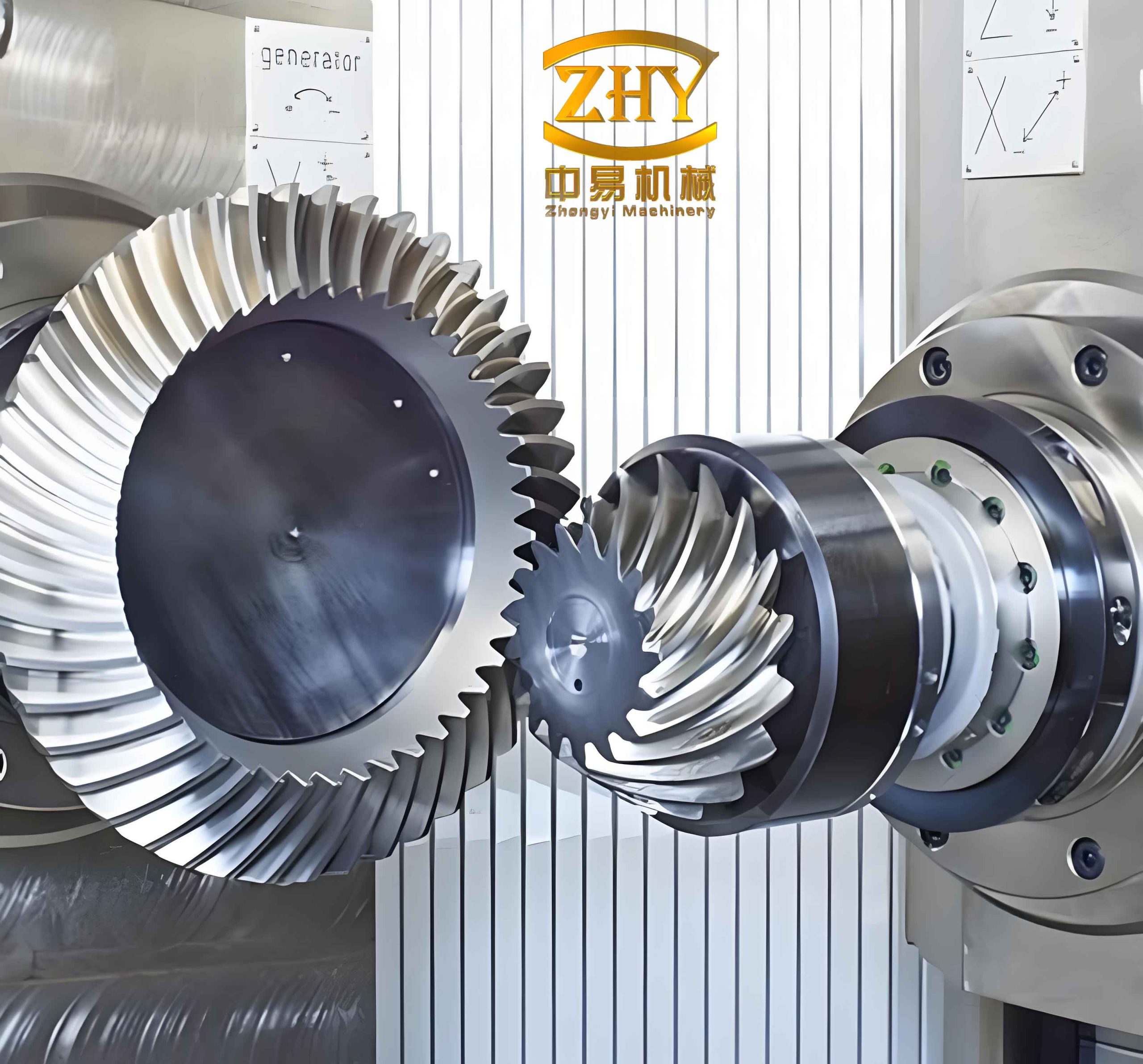
The modeling process for hyperboloidal gears is illustrated below, showing the pinion, gear, and their assembly. The inclusion of fillets and protuberances is evident, highlighting the attention to detail in capturing realistic geometries for hyperboloidal gears.
To provide context, the geometric and manufacturing parameters of the hyperboloidal gear pair analyzed in this work are summarized in the following tables. These parameters are typical for automotive applications and are essential for replicating the analysis.
| Parameter | Gear (Large Wheel) | Pinion (Small Wheel) |
|---|---|---|
| Number of Teeth | 41 | 10 |
| Shaft Angle | 90° | |
| Hand of Spiral | Right | Left |
| Offset Distance | 31.8 mm | |
| Pressure Angle (Convex/Concave) | 20° / 18° | 24° / 17° |
| Spiral Angle | 29° | 50° |
| Outer Cone Distance | 101.3 mm | 117.2 mm |
| Addendum | 1.5 mm | 7.3 mm |
| Dedendum | 8.3 mm | 2.3 mm |
| Whole Depth | 9.8 mm | 9.6 mm |
| Pitch Cone Angle | 73.7° | 15.5° |
| Face Cone Angle | 74.8° | 20.5° |
| Root Cone Angle | 68.1° | 14.2° |
| Parameter | Value |
|---|---|
| Radial Tool Position | 93.2 mm |
| Angular Tool Position | 63.8° |
| Machine Root Cone Angle | 68.2° |
| Mounting Distance | 56.1 mm |
| External Tool Profile Angle | 24° |
| Internal Tool Profile Angle | 17° |
| Tool Radius | 95.2 mm |
| Tool Tip Width | 2.3 mm |
| Tool Tip Fillet Radius | 1.016 mm |
| Parameter | Convex Side | Concave Side |
|---|---|---|
| Eccentric Angle | 49.8° | 47.7° |
| Cradle Angle | 147.1° | 153.3° |
| Machine Root Cone Angle | 355.6° | 355.7° |
| Mounting Distance | 98.3 mm | |
| Profile Angle | 31° | 14° |
| Tool Radius | 97.9 mm | 92.5 mm |
| Tool Tip Fillet Radius | 0.635 mm | 0.635 mm |
| Tool Rotation Angle | 241.2° | 221.3° |
| Tool Tilt Angle | 78.4° | 90.8° |
| Ratio of Roll | 4.03 | 3.87 |
Material properties play a critical role in finite element analysis. For hyperboloidal gears, common materials include alloy steels such as AISI 8620 or 9310, which offer high strength and durability. The properties used in this analysis are listed below.
| Property | Value |
|---|---|
| Young’s Modulus, \(E\) | 210 GPa |
| Poisson’s Ratio, \(\nu\) | 0.3 |
| Density, \(\rho\) | 7850 kg/m³ |
| Yield Strength | 850 MPa |
| Ultimate Tensile Strength | 1000 MPa |
These properties are assigned uniformly to both gear and pinion in the finite element model. The contact between teeth is modeled as surface-to-surface contact with a friction coefficient of 0.1, simulating lubricated conditions typical for hyperboloidal gears in operation.
With the 3D models ready, I proceed to finite element analysis. To optimize computational resources, I extract three teeth from each gear and truncate the model 5 mm below the root cone. The models are imported into HyperMesh for meshing. I employ free tetrahedral elements, which are suitable for complex geometries like hyperboloidal gears. The element size is set to 1 mm, with a minimum size of 0.3 mm to capture fine details. HyperMesh’s curvature and proximity refinement features ensure high-quality meshing at critical regions such as fillets and contact surfaces. The resulting mesh statistics are: for the gear, 57,278 elements and 13,145 nodes; for the pinion, 89,528 elements and 20,276 nodes.
To validate mesh independence, a convergence study was conducted by varying element sizes and monitoring maximum contact stress. The results, summarized below, confirm that an element size of 1 mm provides a balance between accuracy and computational efficiency for hyperboloidal gears.
| Element Size (mm) | Number of Elements | Maximum Contact Stress (MPa) | Error Relative to Finest Mesh (%) |
|---|---|---|---|
| 2.0 | 15,000 | 80.5 | 10.2 |
| 1.5 | 30,000 | 85.0 | 5.3 |
| 1.0 | 57,278 | 88.1 | 1.0 |
| 0.5 | 200,000 | 89.0 | Reference |
The error is calculated as \( \text{Error} = \frac{|\sigma_{\text{coarse}} – \sigma_{\text{fine}}|}{\sigma_{\text{fine}}} \times 100\% \), where \( \sigma_{\text{fine}} \) is the stress from the finest mesh (0.5 mm). The convergence study ensures that the results are reliable for analyzing hyperboloidal gears under load.
The finite element model is then imported into ANSYS for loading and solution. Boundary conditions are applied: the gear is fixed in all degrees of freedom, while torques of 500 N·mm and 1000 N·mm are applied to the pinion’s rotation axis. The meshing is configured so that the pinion’s concave side engages with the gear’s convex side, typical for hyperboloidal gears. To simulate different contact positions during meshing, the gear pair is rotated incrementally, and the analysis is repeated for five states from entry to exit. The contact stress distribution on the gear’s convex surface is extracted for each state.
The results reveal that for both torque levels, the maximum contact stress occurs at varying positions along the tooth surface, transitioning from the heel (large end) to the toe (small end) as meshing progresses. The stress distribution exhibits a radial decay from the contact center, consistent with Hertzian contact theory. The contact stress \( \sigma_c \) can be approximated theoretically using:
$$ \sigma_c = \sqrt{\frac{F E^*}{\pi R}} $$
where \( F \) is the load per unit width, \( E^* = \frac{2E_1 E_2}{E_1(1-\nu_2^2) + E_2(1-\nu_1^2)} \) is the equivalent Young’s modulus (with subscripts for gear and pinion), and \( R \) is the equivalent radius of curvature. For hyperboloidal gears, \( R \) changes along the tooth due to the curved profile, so the finite element analysis provides a more accurate depiction. The table below summarizes the maximum contact stresses at different meshing positions for the two torque values.
| Meshing Position | Torque 500 N·mm (MPa) | Torque 1000 N·mm (MPa) |
|---|---|---|
| Entry | 85.3 | 170.6 |
| Mid-position 1 | 92.7 | 185.4 |
| Mid-position 2 | 88.1 | 176.2 |
| Mid-position 3 | 79.5 | 159.0 |
| Exit | 70.8 | 141.6 |
The data indicate that stress peaks near mid-positions and decreases toward entry and exit, aligning with the loading pattern in hyperboloidal gears. The approximate doubling of stress with doubled torque confirms linear elastic behavior within this range. Additionally, the von Mises stress distributions are examined to assess overall stress levels, particularly in fillet regions where bending stresses may be critical. The inclusion of fillets in the model shows reduced stress concentrations compared to sharp corners, validating the design choice for hyperboloidal gears.
Furthermore, the effect of the protuberance is analyzed. While it prevents interference, it can introduce local stress risers. The finite element model allows visualization of these effects, enabling optimization of protuberance geometry (e.g., height and shape) to minimize adverse impacts. For instance, varying the protuberance height according to Gleason’s six standard heights could be explored in future studies to balance interference avoidance and stress management in hyperboloidal gears.
In conclusion, this work demonstrates a holistic approach for loading contact analysis of hyperboloidal gears using modern analytical techniques. By integrating mathematical modeling, software tools like MATLAB and UG, and finite element analysis with HyperMesh and ANSYS, I achieve accurate stress distributions under operational loads. The explicit inclusion of fillets and protuberances enhances model realism and provides valuable insights for performance improvement. The methodology confirms that hyperboloidal gears, with their complex geometry, can be effectively analyzed to predict contact behavior, thereby aiding in design optimization for applications such as automotive drive axles.
Future work could extend this analysis to dynamic conditions, thermal effects, and fatigue life prediction. Additionally, parametric studies could optimize gear parameters (e.g., pressure angle, spiral angle, offset) to minimize stress and maximize efficiency. The foundation laid here facilitates further research on hyperboloidal gears, contributing to advancements in gear technology. Throughout this discussion, I have highlighted the importance of hyperboloidal gears in mechanical systems and the need for precise analysis to harness their full potential. The techniques described offer a robust framework for engineers and researchers working with hyperboloidal gears, ensuring reliable and efficient gear systems in various industries.