
In my research, I focus on the geometric accuracy and loaded contact mechanical performance of spiral bevel gears manufactured by face milling. The spiral bevel gear is a critical component in power transmission systems, and its tooth surface geometry directly influences load capacity, transmission error, noise, and vibration. Traditional manufacturing optimization often considers only geometric accuracy, but I propose a collaborative optimization framework that integrates both geometric precision and loaded contact mechanical performance. This framework is driven by adaptive data and employs an improved tooth contact analysis (TCA) and a new loaded gear contact analysis (NLTCA). The method is particularly suited for non-orthogonal spiral bevel gears and hypoid gears produced by dual helical face milling. In the following sections, I describe the kinematic model, the initial contact point determination, the NLTCA formulation, the adaptive data-driven collaborative optimization, and a numerical example that validates my approach.
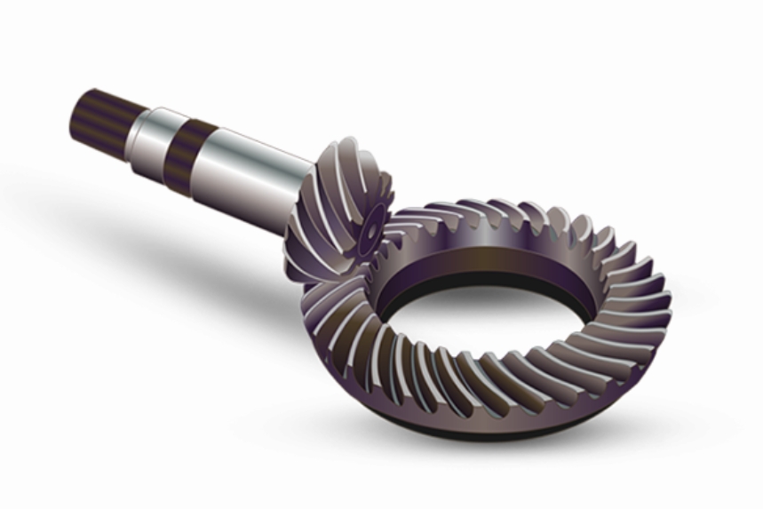
The spiral bevel gear and hypoid gear are widely used in aerospace, automotive, and industrial machinery. Their tooth surfaces are complex, and the manufacturing process involves numerous machine settings. My work addresses the challenge of simultaneously optimizing tooth surface geometric accuracy and loaded contact performance. I use a dual helical face milling method to simulate the generation motion, and I establish a data-driven relationship between assembly errors and loaded contact mechanical performance. The optimization model is adaptive, meaning that it iteratively corrects assembly errors based on sensitivity analysis. I employ a multi-objective optimization (MOO) technique with an achievement function to obtain Pareto optimal solutions. The numerical results demonstrate that my method achieves excellent tooth surface geometric accuracy and improved loaded contact performance for the spiral bevel gear.
Kinematic Model of Dual Helical Face Milling
In my modeling approach, the entire generation motion for the spiral bevel gear is represented by a series of coordinate transformations. The tooth point vector on the gear blank is obtained from the cutter vector through a transformation matrix. For the spiral bevel gear, I use the tilt method for the gear and the dual helical method for the pinion. The general equation for the tooth surface is:
$$ \mathbf{r}_b(\mu,\theta,\phi) = \mathbf{M}_{b-c}(R_a, S_r, E_M, X_D, X_B, \gamma_m, \sigma, \zeta: \phi) \cdot \mathbf{r}_c(\mu,\theta) $$
Here, \(\mathbf{r}\) denotes the tooth point vector, \(b\) denotes the gear, and \(c\) denotes the cutter. The design variables \((\mu,\theta,\phi)\) include the Gaussian parameters \((\mu,\theta)\) and the motion parameter \(\phi\). Under the universal motion concept (UMC), the machine settings include the rotation angle \(\zeta\), tilt angle \(\sigma\), cutter radial setting \(S_r\), rolling ratio \(R_a\), and other parameters. Each parameter can be expressed as a polynomial function of the basic motion parameter \(\phi\). The complex motion chain \(\mathbf{M}_{b-c}\) is given by:
$$ \mathbf{M}_{b-c} = \mathbf{M}_{b-q} \cdot \mathbf{M}_{q-n} \cdot \mathbf{M}_{n-m1} \cdot \mathbf{M}_{m1-p} \cdot \mathbf{M}_{p-w} \cdot \mathbf{M}_{w-c} $$
The relative velocity between the cutter and the work gear blank is essential for the generation motion. At each cutting point position, an additional helical motion exists. The relative velocity \(\mathbf{v}^{(c-b)}\) is expressed as:
$$ \mathbf{v}^{(c-b)}(\mu,\theta,\phi) = (\boldsymbol{\omega}^{(c)} – \boldsymbol{\omega}^{(b)}) \times \mathbf{r}_{m1b}(\mu,\theta,\phi) + \mathbf{O}_1\mathbf{O}_2 \times \boldsymbol{\omega}^{(b)} + \begin{bmatrix} 0 \\ 0 \\ x_{HL}/R \end{bmatrix} a $$
The position vectors and angular velocities are related by the following equations:
$$ \mathbf{r}_{m1b}(\mu,\theta,\phi) = \mathbf{M}_{m1-p} \cdot \mathbf{M}_{p-w} \cdot \mathbf{M}_{w-c} \cdot \mathbf{r}_c(\mu,\theta) $$
$$ \mathbf{O}_1\mathbf{O}_2 = \begin{bmatrix} 0 \\ -E_m \\ X_B \end{bmatrix}, \quad \boldsymbol{\omega}_c = -\begin{bmatrix} 0 \\ 0 \\ R_a \end{bmatrix} = \boldsymbol{\omega}^{(c)}/\boldsymbol{\omega}^{(b)}, \quad \boldsymbol{\omega}^{(b)} = \begin{bmatrix} \cos(\gamma_m) \\ 0 \\ \sin(\gamma_m) \end{bmatrix} $$
Here, \(\mathbf{O}_2\) is the origin of the workpiece coordinate system, and \(\mathbf{O}_1\) is the origin of the cutter coordinate system. The normal vector of the tooth flank point is:
$$ \mathbf{n}_b(\mu,\theta,\phi) = \mathbf{T}_{m1-p} \cdot \mathbf{T}_{p-w} \cdot \mathbf{T}_{w-c} \cdot \mathbf{n}_c(\mu,\theta) $$
where \(\mathbf{T} \in \mathbb{R}^{1 \times 3}\) represents the transformation submatrix of \(\mathbf{M}\). To obtain an accurate spiral bevel gear model, the meshing equation must be satisfied:
$$ f(\mu,\theta,\phi) = \mathbf{n}_b(\mu,\theta,\phi) \cdot \mathbf{v}^{(c-b)}(\mu,\theta,\phi) = 0 $$
This equation ensures that the generating motion produces the correct tooth surface for the spiral bevel gear. I use these equations to simulate the dual helical face milling process and to generate the tooth surface points that will be used in the subsequent contact analysis.
Improved Tooth Contact Analysis for Initial Contact Point Determination
To analyze the loaded contact performance of the spiral bevel gear, I first determine the initial contact points using an improved TCA method that accounts for assembly errors. I consider the small shaft angle of non-orthogonal spiral bevel gears and hypoid gears. The TCA kinematic initialization assumes that the pinion rotation axis is the \(X_2\) axis, located in the positive half-axis domain of the original tooth surface modeling coordinate system \((X_2, Y_2, Z_2)\). Similarly, the gear rotation axis is the \(Z_1\) axis, located in the positive half-axis domain of \((X_1, Y_1, Z_1)\). Because the shaft angle is small, the pinion rotation axis is rotated by \(90^\circ\) around the \(Z_2\) axis, and the current rotation axis is converted to the \(Z_2\) axis. The transformation matrix is:
$$ \mathbf{M}_{X2-Z2} = \begin{bmatrix} \cos(\pi/2) & 0 & \sin(\pi/2) & 0 \\ 0 & 1 & 0 & 0 \\ \sin(\pi/2) & 0 & \cos(\pi/2) & 0 \\ 0 & 0 & 0 & 1 \end{bmatrix} $$
I propose a new pinion tooth surface equation in the contact coordinate system:
$$ \mathbf{r}_2^{[\Theta]}(\mu,\theta,\phi) = \mathbf{M}_{X2-Z2} \cdot \mathbf{r}_b(\mu,\theta,\phi) = \mathbf{M}_{X2-Z2} \cdot \mathbf{M}_{b-c}(\phi) \cdot \mathbf{r}_c(\mu,\theta) $$
Considering the remaining initial meshing calculations, the gear and pinion must be positioned as close as possible in the assembly position. I use the midpoints of the gear and pinion teeth, \(\mathbf{G}_{Mid}(\mu,\theta,\phi)\) and \(\mathbf{P}_{Mid}(\mu,\theta)\), as reference points. The pinion reference point is rotated to the negative half-axis of the \(Y_2\) axis, and the gear reference point is rotated to the positive half-axis of the \(Y_1\) axis. To achieve the precise assembly position, the tooth surface is rotated. The pinion is rotated counterclockwise around the \(Y_2\) axis to the assembly position using the matrix:
$$ \mathbf{M}_{Y2-A2} = \begin{bmatrix} \cos\alpha & 0 & \sin\alpha & 0 \\ 0 & 1 & 0 & 0 \\ -\sin\alpha & 0 & \cos\alpha & 0 \\ 0 & 0 & 0 & 1 \end{bmatrix} $$
The new tooth flanks in the assembly position are:
$$ \mathbf{r}_2^{[\Theta]}(\mu,\theta,\phi) = \mathbf{M}_{Y2-A2} \cdot \mathbf{M}_{PMid-Y2} \cdot \mathbf{M}_{X2-Z2} \cdot \mathbf{r}_b(\mu,\theta,\phi) $$
$$ \mathbf{r}_{G-1}^{[\Theta]}(\mu,\theta,\phi) = \mathbf{M}_{GMid-Y1} \cdot \mathbf{M}_{b-c}(\phi) \cdot \mathbf{r}_c(\mu,\theta) $$
In the assembly position, the two tooth flanks are very close, and the following geometric constraints exist:
$$ (H_{Ad})_{i=1,2} = \frac{1}{2}H_k \pm \lambda_{IP}m $$
$$ (H_{De})_{i=1,2} = H_t – (H_{Ad})_{i=1,2}, \quad \text{when } H_t > H_k $$
Here, \(H_{Ad1}\) and \(H_{Ad2}\) are the gear and pinion addendum, \(H_{De1}\) and \(H_{De2}\) are the gear and pinion dedendum, \(H_t\) is the total tooth height, \(H_k\) is the working tooth height, \(\lambda_{IP}\) is the modification coefficient for initial point determination, and \(m\) is the module. The following relationship holds:
$$ (H_{Ad})_{i=1,2} – (H_{De})_{i=1,2} = H_k – H_t – 2\lambda_{IP}m < 0 $$
To move the intersection point of the tooth surface with the \(Y\) axis downward, I assume that the gear rotation angle equals the pinion rotation angle:
$$ \phi_{G}^{INT}[P_1^*(\mu,\theta,\phi)] = \phi_{G}^{INT}[P_2^*(\mu,\theta,\phi)] $$
I rotate the gear contact surface to the initial contact meshing position using the transformation matrix:
$$ \mathbf{M}_{GMesh} = \begin{bmatrix} \cos(\phi_G) & -\sin(\phi_G) & 0 & 0 \\ \sin(\phi_G) & \cos(\phi_G) & 0 & 0 \\ 0 & 0 & 1 & 0 \\ 0 & 0 & 0 & 1 \end{bmatrix} $$
The new gear tooth surface position is:
$$ (\mathbf{r}_{G-1}^{[\Theta]})^*(\mu,\theta,\phi) = \mathbf{M}_{GMesh} \cdot \mathbf{M}_{GMid-Y1} \cdot \mathbf{M}_{b-c}(\phi) \cdot \mathbf{r}_c(\mu,\theta) $$
Because of the small shaft angle of non-orthogonal gear transmission, the pinion position is determined by:
$$ (\mathbf{r}_{P-1}^{[\Theta]})^*(\mu,\theta,\phi) = [\mathbf{r}_{P-1}^{[\Theta]}(\mu,\theta,\phi) \cdot \mathbf{I}_e] \cdot \mathbf{r}_{P-2}^{[\Theta]}(\mu,\theta,\phi) + \sin(\phi_P) \cdot [\mathbf{I}_e \times \mathbf{r}_{P-1}^{[\Theta]}(\mu,\theta,\phi)] + \cos(\phi_P) \cdot [\mathbf{I}_e \times \mathbf{r}_{P-2}^{[\Theta]}(\mu,\theta,\phi)] \times \mathbf{I}_e $$
where \(\mathbf{I}_e\) is the unit vector of the rotation direction. The TCA equations for determining the initial contact point are:
$$ f_{TCA}(\mu_P,\theta_P,\phi_P,\mu_G,\theta_G,\phi_G) = 0 $$
$$ \text{s.t. } \phi_{G}^{INT} = \phi_{P}^{INT} $$
The contact point calculation involves iterative steps: increasing the positive direction contact points, decreasing the negative direction contact points, terminating when contact points exceed the actual tooth surface, and determining the required contact pattern region \(\Omega_{CP}\). The corresponding TCA evaluations, including contact path and transmission error, are computed directly from the data-driven function relationship. This improved TCA method provides a robust foundation for the subsequent loaded contact analysis of the spiral bevel gear.
Loaded Contact Mechanical Performance via NLTCA
I employ a new loaded gear contact analysis (NLTCA) method based on Hertz contact theory to evaluate the loaded contact mechanical performance of the spiral bevel gear produced by dual helical face milling. When an input torque \(T_{IN}\) is applied to the driving gear shaft, the contact force \(F_K\) at a loaded contact point \(P_{I-J}(\theta,\phi)\) is given by:
$$ T_{INP} = F_K (r_K \cos\alpha_K \cos\beta_K) $$
where \(F_K\) is the force distributed on different tooth flanks, \(r_K\) is the loaded contact point vector, and \(\alpha_K\) and \(\beta_K\) are the profile angle and spiral angle. When two pairs of tooth flanks are in loaded contact, the driven gear rotation angle of the front tooth flank equals the front tooth flank rotation angle. Moreover, the driving rotation angle of the latter is larger than that of the former by a period of \(2\pi/z_1\). Therefore, the following relationships exist:
$$ F_{K-1}(r_{K-1} \cos\alpha_{K-1} \cos\beta_{K-1}) + F_{K-2}(r_{K-2} \cos\alpha_{K-2} \cos\beta_{K-2}) = T_{INP} $$
$$ (\Delta\phi_2)_{LTE}^{[1]}(F_{K-1},\phi_1) + \frac{z_2}{z_1}\phi_1 = (\Delta\phi_2)_{LTE}^{[2]}(F_{K-2},\phi_1 + \frac{2\pi}{z_1}) + \frac{z_2}{z_1}\phi_1 $$
Here, \(z_1\) is the pinion tooth number, \(z_2\) is the gear tooth number, \(\phi_1\) is the pinion rotation angle, and the change in the driven gear rotation angle is represented by the loaded transmission error \((\Delta\phi_2)_{LTE}\). In this contact, “1” denotes the first pair of contact surfaces, and “2” denotes the second pair. When the load acts on each loaded tooth contact point position, the tooth contact deformation considering tooth flexibility \(C_K\) is calculated as:
$$ \omega_K^{(1)} = \sum_{j=1}^{N} C_{Kj}^{(1)} F_j, \quad \omega_K^{(2)} = \sum_{j=1}^{N} C_{Kj}^{(2)} F_j $$
where \(\omega_K^{(1)}\) is the elastic deformation of the pinion, and \(\omega_K^{(2)}\) is the elastic deformation of the gear. In the NLTCA solution, the matching gear contact points are determined by intercepting the two meshing tooth flanks with a normal plane. At each tooth contact position, the following compatibility condition exists:
$$ \omega_K^{(1)} + \omega_K^{(2)} + D_K – \Theta \ge 0 \quad (K=1,2,\dots,N) $$
where \(D_K\) is the initial distance, and \(\Theta\) is the corresponding distance under load. The equality indicates contact state, while the inequality indicates no contact state. The system can be written in matrix form:
$$ \sum_{j=1}^{N} (C_{Kj}^{(1)} + C_{Kj}^{(2)}) F_j + D_K – \Theta \ge 0 \quad (K,j=1,2,\dots,N) $$
In the tooth contact state, all contact point forces \(F_K\) equal all external loads, so the equilibrium equation is:
$$ \{e\}^T \{F\} = T_{INP} $$
By introducing slack variables \(Y\), the equation is rewritten as:
$$ [C]\{F\} + \{D\} – \Theta e – [I]\{Y\} = \{0\} $$
where:
$$ \{Y\} = \{Y_1, Y_2, \dots, Y_K, \dots, Y_N\}^T $$
$$ [I] = \begin{bmatrix} 1 & 1 & 1 & \dots & 1 \end{bmatrix} \in \mathbb{R}^{N \times N} $$
To solve the tooth contact condition, the following relationships must hold:
$$ Y_K = 0, F_K \ge 0; \quad Y_K = 0, F_K \ge 0 $$
I use an improved simplex method to solve the NLTCA equations as a general linear programming problem:
$$ Z_0 = \sum_{j=1}^{N+1} Z_j = Z_1 + Z_2 + \dots + Z_N + Z_{N+1} $$
$$ \text{s.t. } -[C]\{F\} + \Theta e + [I]\{Z\} = \{D\} $$
$$ \{e\}^T \{F\} + Z_{N+1} = T_{INP} $$
$$ Y_K = 0, F_K \ge 0; \quad Y_K = 0, F_K \ge 0 $$
For the \(N+1\) scalar equations, a series of non-negative variable parameters \(Z = [Z_1, Z_2, \dots, Z_N, Z_{N+1}]\) are introduced to make the constant terms on both sides of the equality constraints non-negative. This NLTCA method provides the loaded contact pressure, loaded contact stress, loaded contact pattern, and loaded transmission error for the spiral bevel gear.
Adaptive Data-Driven Collaborative Optimization
I use assembly errors as the basic data for collaborative optimization. The assembly errors \([P, G, e, \alpha]\) are defined as follows: \(P\) represents the displacement of \(O_P\) in the pinion axis direction, \(G\) represents the displacement of \(O_G\) in the gear axis direction, \(e\) represents the offset between the two gear axes, and \(\alpha\) represents the angle between the two gear axes. The positive direction is denoted by “+”, and the negative direction by “−”. The relationship between assembly errors and tooth surface parameters is:
$$ f[\mu(G,P,e,\alpha), \theta(G,P,e,\alpha), \phi(G,P,e,\alpha)] \rightarrow f_p(G,P,e,\alpha) $$
The assembly error \((G,P,e,\alpha)\) can replace machine settings in the correction process, and assembly error correction is an adaptive data-driven design. I establish the following adaptive data-driven collaborative optimization model for dual helical face milling:
$$ [(f_p)^{[0]}(G,P,e,\alpha) – (f_p)_{MOO}^{[\Omega]}(G,P,e,\alpha)] \cdot \mathbf{n}(G,P,e,\alpha) = \mathbf{h} $$
This is transformed into a nonlinear least squares problem:
$$ (G,P,e,\alpha)^{[*]} = \arg\min F(G,P,e,\alpha) = \arg\min \frac{1}{2} \mathbf{h}^T(G,P,e,\alpha) \mathbf{h}(G,P,e,\alpha) $$
The goal is to obtain accurate assembly errors \((G,P,e,\alpha)^{[*]}\), which is actually a feedback and optimization of the initial assembly errors \((G,P,e,\alpha)^{[0]}\) by approximating the target tooth surface. The target tooth surface is determined by the MOO solution. To obtain a robust solution, I use the classic achievement function method for solving MOO problems:
$$ \min W[\omega; (G,P,e,\alpha)] = \min \sum_{j=1}^{k} \omega_j F_j(G,P,e,\alpha) $$
where \(\omega = (\omega_1, \dots, \omega_k)\), such that \(\omega_j \ge 0\) for \(j=1,\dots,k\), and their sum is 1. I assume that all objective functions \(F_j(G,P,e,\alpha)\) for \(j=1,2,3,4\) are scaled to a relative proportion by the transformation:
$$ (f_p)_j^{REL} = F_j^{REL}(G,P,e,\alpha) = \frac{F_j(G,P,e,\alpha) – (f_p)_j^L}{(f_p)_j^U – (f_p)_j^L} \times 100\% $$
The selected achievement function \(S(F \rightarrow \mathbb{R})\) is minimized as:
$$ \min S[F_j, (G,P,e,\alpha)] \rightarrow S[P][F_j, (G,P,e,\alpha); \rho, \omega] $$
where \(\rho > 1\). The final MOO problem is:
$$ [F_j, (G,P,e,\alpha); \rho, \omega] = -\sum_{j=1}^{k} \{\omega_j [F_j(G,P,e,\alpha) – F_j^*]\}^2 + \rho \sum_{j=1}^{k} \max\{0, \{\omega_j [F_j(G,P,e,\alpha) – F_j^*]\}\}^2 $$
Since all maxima of \(S(F \rightarrow \mathbb{R})\) correspond to Pareto optimal solutions of \((G,P,e,\alpha)^* \in PS\), because it is monotonic with respect to the partial order of the objective space, the coefficients are typically \(\omega_j = 0.25\) for \(j=1,2,3,4\), and \(\rho = 1.35\). After determining the Pareto optimal solution corresponding to a given reference point, the interactive step is performed by determining the Pareto frontier \((G,P,e,\alpha)^* \in PF\) of the proposed method.
The collaborative optimization decision is divided into two subsystems. The first subsystem is the loaded contact mechanical performance MOO for target tooth surface determination. The MOO problem is expressed as:
$$ f_{MOO}(G,P,e,\alpha) = \begin{pmatrix} f_1 \\ f_2 \\ f_3 \\ f_4 \end{pmatrix} = \begin{pmatrix} (f_{CP})_{MAX}(G,P,e,\alpha) \\ (f_{LTE})_{MAX}(G,P,e,\alpha) \\ (f_{LCP})_{MAX}(G,P,e,\alpha) \\ (f_{LCS})_{MAX}(G,P,e,\alpha) \end{pmatrix} \rightarrow f_{MOO}^{\Omega}(G,P,e,\alpha) $$
Here, the loaded contact mechanical performance evaluations are selected as the maximum contact pattern \(CP_{MAX}\), including unloaded and loaded contact, the maximum loaded transmission error \(LTE_{MAX}\), the maximum loaded contact pressure \(LCP_{MAX}\), and the loaded contact stress \(LCS_{MAX}\). The second subsystem is the tooth surface geometry optimization through assembly error correction. After the target tooth surface is determined, I use sensitivity analysis of the assembly errors to the ease-off and select a small number of assembly errors as design variables. At each tooth surface point position, I determine the \(n \times m\) sensitivity coefficients for each assembly error, where \(n\) is the number of row tooth points and \(m\) is the number of column tooth points. The average value of the assembly errors is used for result comparison. The larger sensitivity coefficients are selected as the optimization design variables, and their number is usually less than 3. The sensitivity coefficient is calculated as:
$$ S_{[I-J]}(G,P,e,\alpha) = \begin{bmatrix} \frac{\partial [\mathbf{h}(G,P,e,\alpha)]_1}{\partial (G,P,e,\alpha)_1} & \dots & \frac{\partial [\mathbf{h}(G,P,e,\alpha)]_1}{\partial (G,P,e,\alpha)_J} \\ \vdots & \ddots & \vdots \\ \frac{\partial [\mathbf{h}(G,P,e,\alpha)]_I}{\partial (G,P,e,\alpha)_1} & \dots & \frac{\partial [\mathbf{h}(G,P,e,\alpha)]_I}{\partial (G,P,e,\alpha)_J} \end{bmatrix} \quad (I \in [1,n], J \in [1,m]) $$
The basic flow of the adaptive data-driven collaborative optimization considering geometric and loaded contact mechanical performance is as follows: first, the initial assembly errors are used to generate the tooth surface; second, the TCA and NLTCA are performed to evaluate the loaded contact performance; third, the MOO is solved to determine the target tooth surface; fourth, the sensitivity analysis is conducted to select the design variables; fifth, the assembly errors are corrected to minimize the deviation from the target tooth surface; and finally, the optimized assembly errors are output. The number of loaded contact mechanical performance evaluations can be determined according to the actual face milling decision and gear transmission requirements. My proposed collaborative optimization method can be used for non-orthogonal dual helical face milling of spiral bevel gears and hypoid gears.
Numerical Example and Validation
I validate my method using a numerical example of a non-orthogonal spiral bevel gear under heavy-load conditions. The basic geometric design parameters are listed in Table 1. The initial assembly errors are \((G,P,e,\alpha)^{[0]} = [0.25 \text{ mm}, -0.20 \text{ mm}, 0.05 \text{ mm}, 1.0^\circ]\). Table 2 gives the machine settings for the dual helical face milling. Based on the basic design parameters, I model the gear and pinion tooth surfaces and simulate the detailed dual helical face milling considering the initial assembly errors.
| Parameter | Pinion | Gear |
|---|---|---|
| Number of teeth | 31 | 38 |
| Mean normal module (mm) | 5.3 | 5.3 |
| Face width (mm) | 32 | 32 |
| Pressure angle (°) | 22.5 | 22.5 |
| Outer cone distance (mm) | 208.81 | 208.81 |
| Root angle (°) | 22.4 | 27.733 |
| Spiral angle (°) | 23.167 | 28.833 |
| Spiral direction | RH | LH |
| Addendum (mm) | 5.09 | 3.44 |
| Dedendum (mm) | 4.65 | 6.30 |
| Assembly error G (mm) | 0.25 | |
| Assembly error P (mm) | -0.20 | |
| Assembly error e (mm) | 0.05 | |
| Assembly error α (°) | 1.0 | |
| Machine setting | Gear | Pinion |
|---|---|---|
| Cutter radial setting Sr (mm) | 164.02 | 164.13 |
| Workpiece offset Em (mm) | 0 | 0.13 |
| Sliding base setting XB (mm) | -3.96 | -3.33 |
| Cutter root angle γm (°) | 27.73 | 20.13 |
| Blade tilt angle σ (°) | 0.63 | 3.44 |
| Blade rotation angle ζ (°) | 14.83 | 2.54 |
The tooth surface data-driven modeling of the non-orthogonal spiral bevel gear includes the working tooth surface and the root fillet. On the working tooth surface, tooth points are sampled at \(5 \times 9\). In the root fillet working area, tooth points are sampled at \(9 \times 10\) to clearly represent the tooth surface curvature characteristics. After determining the tooth flank points, they can be input into three-dimensional drawing software to generate the solid model. The TCA evaluation items determined by considering assembly errors include the loaded contact path size, position, and direction, which are limited within the constraint boundaries according to the reference standard ANSI/AGMA 2005-D03. The peak-to-peak maximum transmission error is 21.364 \(\mu\)rad, indicating low transmission noise and vibration. After performing MOO on the loaded contact mechanical performance evaluations, the NLTCA evaluation results are determined. First, considering the time-varying meshing characteristics, I determine the loaded contact pressure and its distribution within one period. The instantaneous contact point at each moment is approximately an ellipse, and the loaded contact pressure at the center of the loaded contact point position is maximum. Considering the actual situation of aviation gear transmission, the input torque is 357.5 N·m. Throughout the meshing cycle, the loaded contact pressure changes stably. The larger loaded contact pressures are mainly concentrated in the middle region. At \(T_1 = 3.31\) s, there is no edge contact or concentration phenomenon in the loaded contact pressure, and the distribution is uniform. The maximum value is 420.486 MPa, and the minimum value is 330.852 MPa. At \(T_4 = 3.46\) s, the \(LCP_{MAX}\) at the 5th loaded contact point position during the entire loaded contact meshing process is 1163.10 MPa. At the end of \(T_6 = 3.56\) s, the distribution is relatively uniform, with no edge contact or concentration phenomenon.
When the input torque is 357.5 N·m, Table 3 compares the loaded contact mechanical performance evaluation results before and after the proposed MOO method. In the calculation of the loaded contact pattern, the contact area is greatly increased. After the proposed MOO method, \(LTE_{MAX}\) is reduced by about 44.9%, \(LCP_{MAX}\) is increased by about 13.2%, and \(LCS_{MAX}\) is increased by about 13.9%, which meets the transmission performance requirements.
| Parameter | Before | Proposed MOO method | Change |
|---|---|---|---|
| CPMAX (mm²) | 31.7 | 48.4 | ↑47.4% |
| LTEMAX (m·rad) | 123.5 | 68.1 | ↓44.9% |
| LCPMAX (MPa) | 1026.9 | 1165.3 | ↑13.2% |
| LCSMAX (MPa) | 1841.5 | 2095.3 | ↑13.9% |
In the tooth flank geometric accuracy verification of the non-orthogonal aviation spiral bevel gear and hypoid gear, the main approach is to optimize the assembly error correction by selecting a small number of assembly error evaluations as design variables. First, I determine the sensitivity coefficients of each assembly error evaluation. At the \(5 \times 9\) tooth flank points, the sensitivity coefficients differ greatly. Compared with the average value, the sensitivity coefficient of \(P\) is the largest, followed by \(G\), then \(e\), and finally \(\alpha\). Therefore, \(P\) and \(G\) can be selected as the evaluation optimization design for optimal assembly error correction. To verify the accuracy and robustness of the proposed method, after performing MOO on the loaded contact mechanical performance, I consider different strategies for optimization correction. I consider the ease-off before and after collaborative optimization with different strategies. For different strategy methods, the assembly error corrections are: Case 1: overall optimization using four assembly errors \(P, G, e, \alpha\); Case 2: optimization using three evaluation methods \(P, G, e\); Case 3: optimization using one evaluation method \(P\). Before performing collaborative optimization, numerical comparisons are made with the ease-off values. Before optimization, the mean ease-off is 0.05195 mm, the maximum is 0.07869 mm, the minimum is 0.0000478 mm, and the overall distribution trend varies greatly, with the maximum at the boundary region. The results show that the optimization effect of Case 2 is better than Case 1, and Case 1 is better than Case 3. In summary, the adaptive data-driven collaborative optimization of geometric and loaded contact mechanical performance using three assembly error evaluations \(P, G, e\) as optimization design variables has the best tooth surface geometric accuracy. Finally, to reflect the computational efficiency of the proposed optimization method, I compare the convergence of three data-driven collaborative optimization cases. Although Case 3 has the best computational iteration convergence, it is not the final optimal method because the tooth surface geometric accuracy is unqualified. Case 2 has better convergence than Case 1. Therefore, it can be determined that Case 2 optimization can obtain the best optimization effect.
After determining the tooth surface geometric accuracy of the dual helical face milling, the final task is to output the results and analyze the proposed collaborative optimization. Table 4 shows the output results before and after the adaptive data-driven collaborative optimization considering different strategies. Under the given different sensitivity analysis strategies, their final precise assembly evaluations of the correction amounts are determined. The “[+]” indicates the optimal design variables selected in my method. After comprehensive analysis, Case 2 is the final optimization method due to its high computational accuracy, high efficiency, and good robustness. The final determined output results are the precise assembly errors \((G,P,e,\alpha)^{[*]} = [0.1532 \text{ mm}, -0.0929 \text{ mm}, 0.07861 \text{ mm}, 1.0^\circ]\) plus the correction amounts \((\Delta G, \Delta P, \Delta e, \Delta \alpha) = [-0.0968 \text{ mm}, 0.071 \text{ mm}, 0.02861 \text{ mm}, 0^\circ]\). These assembly errors can be used as inputs for collaborative optimization to ensure good tooth surface geometric accuracy and loaded contact mechanical performance evaluation for the spiral bevel gear.
| Parameter | Before optimization | Case 1 optimized value | Case 2 optimized value | Case 3 optimized value |
|---|---|---|---|---|
| G (mm) | 0.25 | 0.13 (+) | 0.15 (+) | 0.25 |
| P (mm) | -0.20 | -0.11 (+) | -0.10 (+) | -0.08 (+) |
| e (mm) | 0.05 | 0.08 (+) | 0.08 (+) | 0.05 |
| α (°) | 1.0 | 0.86 (+) | 1.0 | 1.0 |
Conclusion
In my research, I proposed an adaptive data-driven collaborative optimization method for the geometric accuracy and loaded contact mechanical performance of spiral bevel gears produced by dual helical face milling. The main conclusions are as follows. First, for the complex tooth surface geometry of non-orthogonal spiral bevel gears and hypoid gears, I used dual helical face milling for simulation modeling and proposed an improved TCA to solve the gear assembly problem. Second, I used a loaded gear contact analysis method (NLTCA) to determine the data-driven relationship between loaded contact mechanical performance evaluation and assembly errors. Considering the multi-objective optimization (MOO) of loaded contact mechanical performance evaluation, I established an adaptive data-driven collaborative optimization model by correcting assembly error evaluations. Third, the adaptive data-driven collaborative optimization decision process was divided into two subsystems: on one hand, the target tooth surface was determined by MOO of loaded contact mechanical performance evaluation using the achievement function method to obtain the Pareto optimal solution; on the other hand, the tooth surface geometric shape was optimized by assembly error correction, and the sensitivity analysis strategy was used to select the best design variables. This optimization strategy improves the efficiency of the entire adaptive data-driven optimization process. The numerical example demonstrated that my method achieves excellent tooth surface geometric accuracy and improved loaded contact mechanical performance for the spiral bevel gear, with significant reductions in loaded transmission error and increases in contact area, contact pressure, and contact stress. The optimized assembly errors can be directly applied to the manufacturing process to ensure high-quality spiral bevel gear production.