
The performance and longevity of power transmission systems critically depend on the tribological behavior of their components. Among these, the helical gear is a cornerstone of modern machinery, prized for its smooth operation, high load capacity, and reduced noise compared to spur gears. However, the very engagement process that grants these advantages also subjects the tooth flanks to continuous friction and wear. This wear is not merely a superficial concern; it progressively alters the surface topography, redistributes the load, amplifies transmission error, and ultimately precipitates vibration, noise, and catastrophic failure modes. Therefore, developing accurate predictive models for gear wear is paramount for reliable design and maintenance.
Traditionally, wear calculations for gear systems, including the helical gear, have often relied on simplified assumptions. A prevalent approach treats the complex, evolving point or line contact as a series of discrete, static observations, applying the foundational Archard wear model with a constant wear coefficient. While insightful, such models struggle to account for the dynamic realities of meshing: the continuous variation in sliding velocity, contact pressure, and lubrication regime along the contact path. Furthermore, modern design frequently employs intentional modifications—profile shifts (modification) and topological ease-off corrections—to optimize contact patterns and mitigate stress concentrations. These modifications fundamentally change the contact mechanics from ideal line contact to a controlled point contact, rendering traditional line-contact-based wear analyses inadequate. The challenge lies in developing a methodology that seamlessly integrates the geometric definition of a modified tooth surface with a dynamic, physics-based wear calculation.
This article addresses this challenge by presenting a comprehensive, integrated methodology for calculating adhesive wear on the tooth flanks of modified helical gears. The core of our approach is the foundation of ease-off topography analysis. From this starting point, we derive the essential meshing parameters. We then employ a discretized quasi-Hertzian point contact model to accurately resolve the contact pressure distribution, even at the edges of the contact zone where stress concentrations occur. Crucially, we abandon the notion of a constant wear coefficient. Instead, we leverage a regression-based model to compute a dynamic wear coefficient for every instant and location on the contacting surfaces, capturing the influence of instantaneous load, curvature, and surface conditions. Finally, we synthesize these elements to compute the wear depth distribution across the entire tooth flank over a designated operational life. This integrated workflow, from ease-off definition to three-dimensional wear mapping, provides a powerful theoretical tool for the anti-wear design and precision life prediction of advanced helical gear transmissions.
Geometric Foundation: The Ease-Off Topology and Surface Mapping
The precise definition of the tooth surface geometry is the indispensable first step in any contact or wear analysis. For a modified helical gear, we begin with the concept of an ease-off surface, which is a powerful tool for representing the deviation between the actual manufactured tooth surface and a theoretical reference surface. Consider a basic rack $\Sigma_0$ that is tangent to the helical gear tooth surface. This rack surface serves as a convenient and neutral mapping plane onto which we can project and compare different tooth flank geometries.
Let us define a coordinate system $(u, v, w)$ on this rack plane $\Sigma_0$, where $u$ represents the direction along the face width, $v$ represents the direction along the tooth profile (essentially the trace of the contact line), and $w$ represents the normal deviation from the plane. The surface of a standard, unmodified involute helical gear generated by this rack can be denoted as $\Sigma_s$. When topological modifications are applied during manufacturing—such as lead crowning, profile relief, or twist—the resulting actual tooth surface is different and can be denoted as $\Sigma_i$.
The ease-off surface is precisely the calculated difference between these two surfaces when mapped onto the common rack plane $\Sigma_0$. If we represent the standard surface as $w_s(u,v)$ and the modified surface as $w_i(u,v)$, then the ease-off $\delta(u,v)$ is given by:
$$ \delta(u, v) = w_i(u, v) – w_s(u, v) $$
For a parabolic modification, which is common for achieving a localized bearing contact, the modified surface $w_i(u,v)$ can often be described by a second-order function:
$$ w_i(u,v) = a_0 + a_1 u^2 + a_2 u v + a_3 v^2 $$
In this formulation, the coefficient $a_1$ primarily controls lead crowning (modification along the face width $u$), $a_3$ controls profile relief or modification (along the profile direction $v$), and the cross-term coefficient $a_2$ controls the twist or bias in the contact pattern. The ease-off surface $\delta(u,v)$ thus becomes a three-dimensional map that visually and quantitatively represents the intentional deviation introduced into the helical gear tooth flank.
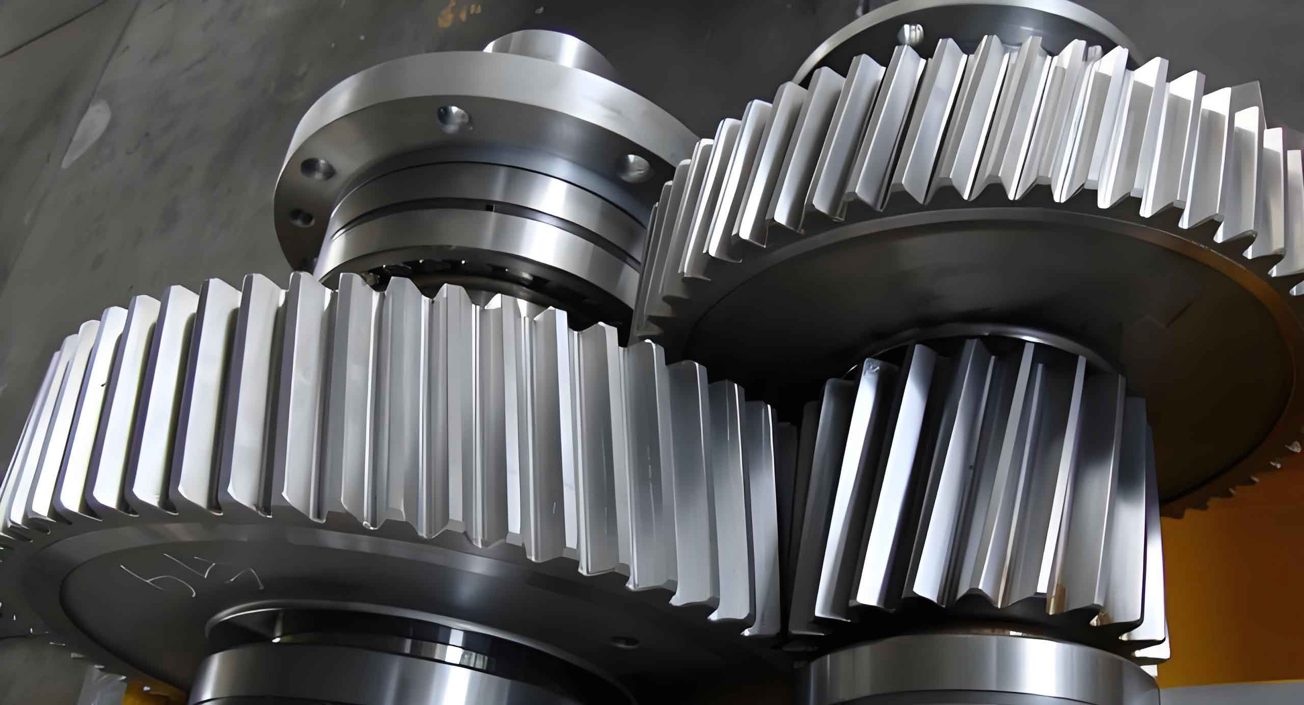
The true power of this representation emerges when considering a gear pair. We can construct an ease-off surface for the pinion (Gear 1) relative to its generating rack, and another for the gear (Gear 2). The composite ease-off surface governing their meshing is not simply one of these, but a function of both. For conjugate meshing analysis, we construct the “ease-off” between the pinion surface and the conjugate of the gear surface (or vice-versa). This final composite ease-off surface encapsulates the combined effect of both gears’ modifications on their contact. The contours and curvature of this surface directly determine the instantaneous contact ellipse’s size, orientation, and path across the tooth flank. Every point on a “difference curve” (a slice of the ease-off surface at a fixed meshing position) corresponds to a potential contact point, and its local geometry provides the crucial curvature data needed for subsequent stress and wear calculations.
Analytical Derivation of Meshing Parameters
With the tooth flank geometry defined via the ease-off topology, we proceed to derive the kinematic and mechanical parameters necessary for wear calculation. These include the principal curvatures for contact mechanics, the sliding ratios, and the resulting sliding distances.
Curvature Parameters and Equivalent Radius
The local curvature at any point on the ease-off surface determines the Hertzian contact conditions. For a point defined by parameters $(u_i, v_i)$ with an ease-off value $z_{di}$, the principal curvatures and directions can be derived using differential geometry. The first and second fundamental forms of the surface are required. Let the surface be defined as $\mathbf{r}(u,v)$. The coefficients of the first fundamental form $E$, $F$, $G$ and the second fundamental form $L$, $M$, $N$ are calculated from the partial derivatives of $\mathbf{r}$.
The normal curvature $\kappa_n$ in a direction given by $du:dv$ is:
$$ \kappa_n = \frac{L\,du^2 + 2M\,du\,dv + N\,dv^2}{E\,du^2 + 2F\,du\,dv + G\,dv^2} $$
By finding the eigenvalues and eigenvectors of the shape operator, we obtain the principal curvatures $\kappa_1$ and $\kappa_2$. For the purpose of contact stress calculation between two surfaces, the equivalent or reduced radius of curvature $R_{bj}$ in the plane of contact (often related to the direction normal to the instantaneous contact line) is the most critical parameter. If the principal relative radii of the gear pair at the contact point are $R_1$ and $R_2$, the equivalent radius $R_{bj}$ is given by:
$$ \frac{1}{R_{bj}} = \frac{1}{R_1} \pm \frac{1}{R_2} $$
where the sign depends on whether the surfaces are convex-convex or convex-concave. This equivalent radius $R_{bj}$ feeds directly into the Hertzian contact equations to determine the contact semi-width and pressure distribution.
Sliding Ratio and Sliding Distance Calculation
Relative sliding between the contacting flanks of a helical gear is the primary driver of adhesive wear. The sliding ratio quantifies this relative motion. A more universal method than traditional geometric formulas involves direct computation from the spatial kinematics of the meshing pair.
Let $\mathbf{\omega}_1$ and $\mathbf{\omega}_2$ be the angular velocity vectors of the pinion and gear, respectively. Let $\mathbf{r}_1$ and $\mathbf{r}_2$ be the position vectors of the instantaneous contact point $K$ in the coordinate systems attached to each gear. The velocities of the contact point on each gear are:
$$ \mathbf{V}_1 = \mathbf{\omega}_1 \times \mathbf{r}_1, \quad \mathbf{V}_2 = \mathbf{\omega}_2 \times \mathbf{r}_2 $$
Let $\mathbf{n}$ be the common unit normal vector to both surfaces at the contact point. The component of velocity along the normal (the entraining or rolling velocity) is the same for both gears to maintain contact:
$$ V_t = \mathbf{n} \cdot \mathbf{V}_1 = \mathbf{n} \cdot \mathbf{V}_2 $$
The tangential sliding velocities for each gear are then:
$$ \mathbf{u}_1 = \mathbf{V}_1 – V_t \mathbf{n}, \quad \mathbf{u}_2 = \mathbf{V}_2 – V_t \mathbf{n} $$
The relative sliding velocity vector is $\mathbf{v}_s = \mathbf{u}_1 – \mathbf{u}_2$. The magnitudes of the tangential velocities $u_1 = |\mathbf{u}_1|$ and $u_2 = |\mathbf{u}_2|$ are used to define the sliding ratios. The sliding ratio for the pinion (Gear 1) is:
$$ \mu_1 = \frac{u_1 – u_2}{u_1} $$
And for the gear (Gear 2), considering the different number of contact cycles, it is:
$$ \mu_2 = i_{21} \cdot \frac{u_1 – u_2}{u_2} $$
where $i_{21}$ is the gear ratio (number of teeth of gear / number of teeth of pinion). The sliding distance, which is the physical length one surface slides over another during the passage of the contact, is proportional to the contact zone size and the sliding ratio. If $a_H$ is the semi-width of the contact ellipse in the direction of sliding, the sliding distances for one engagement are approximately:
$$ s_1 = 2 a_H |\mu_1|, \quad s_2 = 2 a_H |\mu_2| $$
Load Distribution and Quasi-Hertzian Point Contact Solution
Determining the contact pressure distribution is a central challenge, especially for topologically modified helical gears where contact is intentionally localized into an elliptical area. Classic Hertz theory provides solutions for ideal ellipsoidal bodies, but it breaks down when the contact ellipse intersects the boundary of the gear tooth, leading to edge loading and severe stress concentrations. To solve this problem accurately, we adopt a discretized quasi-Hertzian approach.
The instantaneous contact zone predicted by the ease-off analysis is discretized along the potential contact line into a finite number of small, independent slices or elements. Each element, of length $\Delta l$, is treated as a line contact problem between two cylindrical bodies whose radii are defined by the local curvatures from the ease-off surface. The total normal load $F$ is distributed among these $m$ elements: $F = \sum_{j=1}^{m} f_j$.
For each element $j$ carrying a load $f_j$, the load per unit length is $q_j = f_j / \Delta l$. The equivalent radius for that element is $R_{bj}$. The semi-half width $a_{Hj}$ of this hypothetical line contact is given by the Hertzian formula:
$$ a_{Hj} = \sqrt{\frac{4 f_j R_{bj}}{\pi \Delta l E_q}} = \sqrt{\frac{4 q_j R_{bj}}{\pi E_q}} $$
where $E_q$ is the equivalent elastic modulus:
$$ \frac{1}{E_q} = \frac{1-\nu_1^2}{E_1} + \frac{1-\nu_2^2}{E_2} $$
The contact pressure distribution across the width $y$ of this element (ranging from $-a_{Hj}$ to $+a_{Hj}$) is semi-elliptical:
$$ p_j(y) = p_{0j} \sqrt{1 – \frac{y^2}{a_{Hj}^2}}, \quad \text{with} \quad p_{0j} = \sqrt{\frac{q_j E_q}{\pi R_{bj}}} $$
By assembling the pressure distributions from all discrete elements across the contact zone, we construct a complete pressure map $p(u,v)$ that accurately models the true contact, including the rise in pressure at the edges of the tooth flank. This $p(u,v)$ is the key mechanical input for the wear calculation. The following table summarizes the key parameters for the quasi-Hertzian contact model.
| Symbol | Description | Formula / Source |
|---|---|---|
| $R_{bj}$ | Equivalent radius of curvature at element j | Derived from ease-off surface curvature analysis |
| $f_j$ | Normal load on discrete element j | From load distribution solving (e.g., compatibility of deformations) |
| $q_j$ | Load per unit length on element j | $q_j = f_j / \Delta l$ |
| $E_q$ | Equivalent elastic modulus | $1/E_q = (1-\nu_1^2)/E_1 + (1-\nu_2^2)/E_2$ |
| $a_{Hj}$ | Semi-contact width for element j | $a_{Hj} = \sqrt{4 q_j R_{bj} / (\pi E_q)}$ |
| $p_{0j}$ | Maximum Hertzian pressure for element j | $p_{0j} = \sqrt{q_j E_q / (\pi R_{bj})}$ |
The Dynamic Adhesive Wear Calculation Model
With the geometry, kinematics, and contact pressure defined, we can now formulate the wear model. We focus on adhesive wear, which is dominant for gear steel pairs of similar hardness. The foundational model is the Archard wear equation:
$$ V = k \cdot \frac{W \cdot s}{H} $$
where $V$ is the wear volume, $k$ is the dimensionless wear coefficient, $W$ is the normal load, $s$ is the sliding distance, and $H$ is the hardness of the softer material. For computational tractability in predicting wear depth distribution on a helical gear tooth flank, we transition to an incremental depth-based formulation. The incremental wear depth $\Delta h$ at a specific point on the surface for one contact event is:
$$ \Delta h = K_0 \cdot p \cdot s $$
Here, $p$ is the contact pressure at that point (from our quasi-Hertzian solution), $s$ is the sliding distance for that engagement (calculated from kinematics), and $K_0$ is a dynamic wear coefficient with units of $\text{m}^2/\text{N}$. This coefficient is not a constant material property but a variable that depends on the instantaneous local operating conditions.
Determination of the Dynamic Wear Coefficient $K_0$
Assigning a fixed value to $K_0$ is a significant simplification. In reality, it is influenced by lubrication regime, surface roughness, contact pressure, and material properties. We employ a regression model derived from extensive experimental data to estimate $K_0$ dynamically for each contact point. The model is expressed in terms of dimensionless parameters:
$$ K_0 = \frac{3.981 \times 10^{29}}{E_q} \cdot L_1^{1.219} \cdot G_1^{-7.377} \cdot S_1^{1.589} $$
where the dimensionless parameters are defined as follows:
$$
\begin{align*}
L_1 &= \frac{q}{E_q R_b} \quad &\text{(Dimensionless load parameter)} \\
G_1 &= \alpha E_q \quad &\text{(Dimensionless materials parameter)} \\
S_1 &= \frac{R_c}{R_b} \quad &\text{(Dimensionless roughness parameter)}
\end{align*}
$$
In these definitions:
- $q$ is the load per unit length ($q_j$ in our discrete model).
- $E_q$ is the equivalent elastic modulus.
- $R_b$ is the equivalent radius of curvature ($R_{bj}$).
- $\alpha$ is the pressure-viscosity coefficient of the lubricant.
- $R_c$ is the composite surface roughness: $R_c = \sqrt{R_{a1}^2 + R_{a2}^2}$, where $R_{a1}$ and $R_{a2}$ are the arithmetic average roughness of the pinion and gear, respectively.
This formulation directly links the wear coefficient to the instantaneous mechanical and tribological state. For example, a smaller equivalent radius $R_b$ (as often found near the root or tip of a helical gear tooth) leads to a larger $S_1$ and thus a larger $K_0$, indicating a propensity for higher wear in those regions, all else being equal.
Cumulative Wear Calculation and Surface Update
The total wear at any point is the summation of incremental wear over millions of contact cycles. However, as wear accumulates, the surface geometry changes, which in turn alters the contact pressure distribution and sliding conditions. A simple linear summation would eventually become inaccurate. To address this, we implement an iterative wear-life simulation protocol:
- Initialization: Start with the pristine, topologically defined tooth surfaces of the helical gear pair. Set total cycles $N = 0$ and wear depth map $h(u,v) = 0$.
- Single-Cycle Wear Map: For the current geometry, calculate the complete set of meshing parameters, contact pressures $p(u,v)$, sliding distances $s(u,v)$, and dynamic wear coefficients $K_0(u,v)$ for one mesh cycle. Compute the incremental wear depth map $\Delta h(u,v) = K_0(u,v) \cdot p(u,v) \cdot s(u,v)$.
- Wear Accumulation: Add the incremental wear to the total wear map: $h_{\text{new}}(u,v) = h_{\text{old}}(u,v) + \Delta h(u,v)$.
- Surface Update Check: Compare the maximum wear depth increment to a predefined update threshold (e.g., 1-5 $\mu$m). If the threshold is exceeded, proceed to step 5. If not, repeat from step 2 for the next block of cycles until the threshold is met.
- Surface Reconstruction: Update the digital tooth flank model by subtracting the accumulated wear depth $h(u,v)$ from the original surface geometry. This creates a new “worn” ease-off topography.
- Iteration: With the updated geometry, recalculate the meshing parameters (Step 2) and continue the process.
- Termination: The simulation runs until a specified total number of cycles is reached or until the wear depth exceeds a failure criterion (e.g., 5% of the module or a critical loss of profile).
This algorithm ensures that the wear prediction accounts for the dynamic interaction between changing geometry and changing contact mechanics, providing a more realistic life prediction for the helical gear pair.
Analysis of Wear Distribution in a Helical Gear Pair
To demonstrate the methodology, we present a numerical simulation for a helical gear pair with parabolic ease-off modification. The basic parameters of the gear pair are summarized in the table below.
| Parameter | Symbol | Value |
|---|---|---|
| Gear Ratio | $i_{12}$ | 29 / 21 |
| Face Width | $B$ | 80 mm |
| Normal Module | $m_n$ | 5 mm |
| Normal Pressure Angle | $\alpha_n$ | 20° |
| Helix Angle | $\beta$ | 13° |
| Profile Shift Coefficient (Pinion) | $x_1$ | +0.1 |
| Profile Shift Coefficient (Gear) | $x_2$ | -0.098 |
| Young’s Modulus | $E$ | 209 GPa |
| Poisson’s Ratio | $\nu$ | 0.3 |
| Surface Roughness | $R_a$ | 0.2 $\mu$m |
| Lubricant Pressure-Viscosity Coefficient | $\alpha$ | 1.39 $\times 10^{-8}$ m²/N |
| Pinion Speed | $n_1$ | 3000 rpm |
Distribution of Key Parameters
The computed dynamic wear coefficient $K_0$ shows a distinct pattern across the tooth flank of the helical gear. It tends to be higher in the regions of smaller equivalent radius, typically near the root of the pinion and the tip of the gear. Along the face width, it peaks in the central region due to the parabolic crowning which minimizes $R_b$ at the center of the contact path.
The contact pressure $p$ and semi-contact width $a_H$ are intrinsically linked. Their distribution mirrors the ease-off topology. The parabolic lead modification successfully concentrates the load towards the center of the face width, creating a distinct pressure “bullseye.” Due to the profile shift, the region of maximum pressure for the pinion is shifted slightly towards its tip, while for the negatively shifted gear, it is shifted towards its root.
The sliding ratio $\mu$ exhibits the classic pattern for involute gears: it is highest in magnitude at the points of single-pair contact near the root and tip, and passes through zero (pure rolling) near the pitch point. The sliding distance $s$, being the product of $2a_H$ and $|\mu|$, shows a combined influence. It is generally highest where the contact is wide and the sliding ratio is significant, often leading to elevated values in the root region of the pinion and the tip region of the gear.
Predicted Wear Depth Distribution
After simulating $3.0 \times 10^6$ cycles of the pinion, the calculated wear depth distributions for both gears reveal critical insights into the wear behavior of this modified helical gear pair.
Pinion (Gear 1): The wear depth is not uniform. Along the profile direction, wear is most severe near the root, moderate near the tip, and minimal around the pitch circle. This is a direct consequence of high sliding ratios and pressures in the root region. Along the face width, wear is concentrated in the central zone due to the crowning. A significant observation is that the wear gradient is very steep in the engaging-in region (where the pinion root contacts the gear tip), indicating a rapid initial wear process. In contrast, the engaging-out region shows a more uniform wear distribution. This asymmetry can lead to localized pitting or scuffing initiation in the pinion root area.
Gear (Gear 2): The wear pattern on the gear is more symmetrical, resembling a saddle shape. The wear is slightly higher at the gear’s tooth tip than at its root, which contrasts with some simplified models. This occurs because the dynamic wear coefficient $K_0$ is highest at the gear tip (small $R_b$), and while the sliding distance might be higher at the root, the product $K_0 \cdot p \cdot s$ is maximized at the tip in this specific case. The parabolic crowning again focuses wear towards the center of the face width. Edge contact effects at the boundaries of the active flank area can lead to a rapid increase in wear depth, highlighting the importance of proper lead modification to avoid such edge loading in a helical gear.
Parametric Study on Wear
The influence of key design and operational parameters on wear distribution was investigated. The trends are summarized below.
| Parameter Varied | Effect on Pinion Wear | Effect on Gear Wear | Design Implication |
|---|---|---|---|
| Increased Profile Shift ($x_1 \uparrow$, $x_2 \downarrow$) | Wear peak shifts from root towards pitch line; engaging-in wear decreases, engaging-out wear increases. | Wear peak shifts from tip towards pitch line; pattern becomes more uniform. | Selecting appropriate profile shift coefficients can balance and homogenize wear between the pair, extending system life. |
| Increased Torque ($T \uparrow$) | Wear depth increases proportionally more than linearly. High gradients persist at contact zone ends. | Wear depth increases significantly across the entire contact zone. | Overloading dramatically accelerates wear. Design must ensure adequate face width and hardness for the intended load. |
| Increased Gear Ratio ($i_{12} \uparrow$) | Overall wear depth decreases, primarily due to increased equivalent radius reducing $K_0$. | Overall wear depth decreases, primarily due to reduced sliding distance $s_2$. | For a given center distance and pinion size, a larger gear ratio can be beneficial from a wear perspective for the specific gear pair analyzed. |
Conclusion
This article has presented a comprehensive and integrated methodology for calculating adhesive wear on the tooth flanks of ease-off topologically modified helical gears. The method bridges the gap between high-precision gear geometry definition and dynamic tribological analysis. Key contributions and findings include:
- The use of the ease-off surface as the fundamental geometric descriptor provides a unified framework to model modifications (profile shift, lead crowning, twist) and derive all necessary contact geometry parameters for the helical gear.
- The discretized quasi-Hertzian point contact model offers a robust and accurate solution for determining the contact pressure distribution, successfully handling the challenging case of edge contact and stress concentration on the boundaries of the helical gear tooth flank.
- Moving beyond constant wear coefficients, the implementation of a dynamic wear coefficient model based on instantaneous local conditions (load, curvature, roughness) is crucial for realistic wear prediction. This coefficient is highest in regions of small radius of curvature, such as the pinion root and gear tip.
- The predicted wear distribution for a parabolic modified helical gear pair shows distinct patterns: the pinion suffers maximum wear in the root region near the center of the face width, with a severe gradient in the engaging-in zone. The gear experiences slightly higher wear at the tip, also concentrated at the face width center. The wear is minimal near the pitch circle.
- Parametric studies confirm that design choices significantly impact wear life. Proper selection of profile shift coefficients can optimize and balance wear between the mating helical gears. Load (torque) has a strongly non-linear accelerating effect on wear, while increased gear ratio may reduce wear for the specific pair under study.
This methodology, providing a complete workflow from ease-off topology to 3D wear mapping, serves as a powerful theoretical and computational tool. It enables engineers to perform virtual wear-life testing, optimize ease-off topography for minimal and uniform wear, and ultimately design helical gear transmissions with extended precision life and enhanced reliability. Future work may integrate this model with pitting fatigue analysis and thermal-elastic-hydrodynamic lubrication models for an even more complete surface durability prediction.