
Throughout my career in mechanical design and software development, I have often encountered the challenge of creating precise three-dimensional models of worm gears. These components are indispensable in power transmission applications, yet their complex tooth surfaces, governed by strict geometric equations and constraints, make direct manipulation in conventional CAD systems extremely difficult. In this work, I present a comprehensive method to achieve accurate 3D modeling of worm gears by exploiting the ActiveX Automation Interface of Mechanical Desktop 6 (MDT 6.0) through Visual Basic programming. This approach leverages MDT’s native helical sweep functionality, combined with parametric tooth profile definitions, to produce high-fidelity models suitable for design, finite element analysis, manufacturing simulation, and digital twin development.
Introduction to Worm Gears and Modeling Challenges
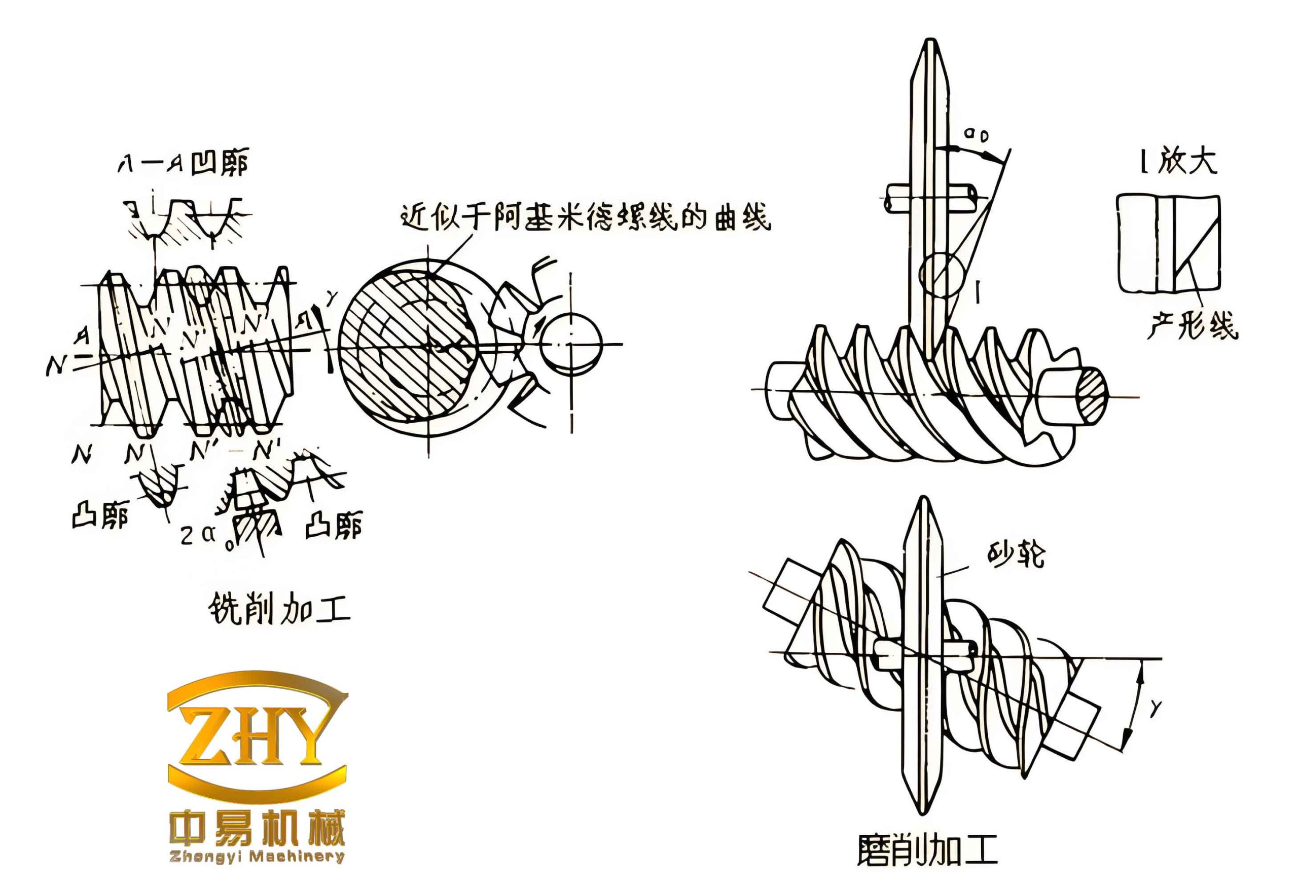
Worm gears are a common type of gear mechanism consisting of a worm (which resembles a screw) and a worm wheel (a helical gear). They offer high reduction ratios, smooth and quiet operation, and self-locking capabilities in many configurations. The tooth surfaces of worm gears must satisfy specific meshing conditions. For cylindrical worm gears, the most prevalent types include the Archimedean worm (ZA), the involute worm (ZI), and the normal straight-sided worm (ZN). Each type is produced by different cutting tool geometries and installation positions, leading to distinct tooth profiles in transverse or normal sections. Modeling these surfaces manually in a 3D environment is error‑prone and labor‑intensive. My solution automates the process through programmatic control of MDT, a powerful add‑on to AutoCAD that excels in parametric solid modeling. By using Visual Basic, a language with a gentle learning curve, I enable engineers to generate worm gear models quickly and accurately without deep expertise in CAD scripting.
Parameterization of Worm Gear Geometry
The foundation of any worm gear model lies in its basic parameters. Let us define the key inputs:
| Symbol | Description | Typical Values / Units |
|---|---|---|
| \(m\) | Module (axial module for worm) | mm |
| \(z_1\) | Number of worm threads (starts) | 1, 2, 3, … |
| \(z_2\) | Number of worm wheel teeth | ≥ 30 typically |
| \(q\) | Worm diameter coefficient | \(q = d_1 / m\) |
| \(\alpha\) | Pressure angle (standard 20°) | degrees |
| \(h_a^*\) | Addendum coefficient | usually 1.0 |
| \(c^*\) | Clearance coefficient | usually 0.25 or 0.2 |
From these, we derive the reference diameters, tip diameters, root diameters, and base circle diameters. For a worm, the lead (axial pitch) is given by:
$$P_z = \pi m z_1$$
The reference diameter of the worm is \(d_1 = m q\), while the reference diameter of the worm wheel is \(d_2 = m z_2\). The center distance becomes \(a = 0.5 m (q + z_2)\). The tooth height dimensions follow standard gear formulas:
$$h_a = h_a^* m, \quad h_f = (h_a^* + c^*) m$$
These parameters are used to compute the coordinates of the cutting tool profiles for both the worm and the worm wheel.
3D Modeling of the Worm
The worm tooth surface is generated by simulating the cutting process on a lathe. A straight‑edged cutting tool is positioned relative to the worm axis according to the worm type. The tool profile is first created as a 2D sketch on a plane that contains the worm axis for ZA worms, or offset by the base radius for ZI worms. I implement the tool geometry using the coordinates computed from the formulas provided in the original work. The key points for a symmetric cutting tool are listed in Table 2.
| Point | X (radial direction) | Y (axial direction) | Description |
|---|---|---|---|
| 1 | 0 | \(m q – (h_a^* + c^*) m\) | Root point on axis |
| 2 | \(c^* m\) | \(Y_1\) | Root fillet start |
| 3 | \(\frac{\pi m}{4} – h_a^* m \tan\alpha\) | \(c^* m + Y_1\) | Tooth flank start |
| 4 | \(\frac{\pi m}{4} + h_a^* m \tan\alpha\) | \((2h_a^* + c^*) m + Y_1\) | Tooth flank end |
| 5 | \(X_4\) | \(1.5 Y_1\) | Top land |
| 6 | 0 | \(Y_5\) | Top point on axis |
The arc between points 1 and 2 is assigned a bulging factor (convexity) of 0.2 via the SetBulge method to represent the root fillet radius. All other segments are straight lines. Using MDT’s object model, I first create a lightweight polyline with AddLightWeightPolyline, then convert it into a sketch with AddSketch. The resulting 2D profile represents the cross‑section of the cutting tool.
Next, a cylindrical blank for the worm is created with diameter equal to the worm outer diameter \(d_a = d_1 + 2 h_a\) and length \(L\) (sufficient to contain the threaded portion). A 3D helical path is defined using the MDT helical sketch descriptor. The parameters of the helix are:
| Parameter | Value |
|---|---|
| Pitch (lead) | \(\pi m z_1\) |
| Number of revolutions | \(L / (\pi m z_1)\) |
| Starting angle | 0° or 90° depending on view orientation |
The cutting profile is then swept along this helical path using the mcSweep feature with CombineType = mcCut. This subtractive operation carves one helical tooth space from the cylindrical blank. For multi‑start worms (e.g., \(z_1 = 2\)), the resulting tooth space feature is replicated using a polar array around the axis with \(z_1\) copies, producing the complete worm geometry. The core programming steps follow:
Create cylindrical blank (extrusion)
Define 3D helical path sketch
Create cutting profile sketch
Invoke sweep cut: Set Profile = cuttingSketch, Path = helicalSketch, CombineType = mcCut
If z1 > 1: polar array the cut feature around axis with count = z1
This method produces a worm with the correct axial tooth profile. For ZI worms, the tool profile is split into left and right halves, each offset from the worm axis by the base circle radius \(r_b = r_1 \cos\alpha_t\), where \(\alpha_t\) is the transverse pressure angle. The two halves are swept separately to form the involute tooth flanks.
3D Modeling of the Worm Wheel
The worm wheel is modeled by a similar subtractive sweep, but this time the cutting tool profile is defined on the face (end) of the cylindrical blank. The tooth space of a worm wheel in the transverse plane follows the shape of a gear with an involute profile modified by the worm’s geometry. The coordinates of the cutting points (shown in the original figure) are computed from the reference circle radius \(R\), tip radius \(R_a\), root radius \(R_f\), and base radius \(R_b\) of the worm wheel. Key formulas include:
$$R = \frac{m z_2}{2}, \quad R_a = R + h_a m, \quad R_f = R – h_f m, \quad R_b = R \cos\alpha$$
The angular parameter \(\theta_3\) that defines the transition point is given by:
$$\theta_3 = \frac{\pi m \cos\alpha – s_b}{2 s_b}$$
where \(s_b\) is the base circle tooth thickness:
$$s_b = \cos\alpha \left( \frac{\pi m}{2} + m z_2 (\tan\alpha – \alpha) \right)$$
Table 4 gives the Cartesian coordinates of the seven key points for the half‑tooth space profile (symmetric about the Y‑axis).
| Point | X | Y | Description |
|---|---|---|---|
| 1 | 0 | \(R_f\) | Root center |
| 2 | \(R_f \sin(\theta_3/3)\) | \(R_f \cos(\theta_3/3)\) | Root fillet |
| 3 | \(R_b \sin\theta_3\) | \(R_b \cos\theta_3\) | Start of involute |
| 4 | \(R \sin(\theta_3 + \tan\alpha – \alpha)\) | \(R \cos(\theta_3 + \tan\alpha – \alpha)\) | Pitch point |
| 5 | \(R_a \sin(\theta_3 + \tan\alpha – \alpha)\) | \(R_a \cos(\theta_3 + \tan\alpha – \alpha)\) | Tip point |
| 6 | \(X_5\) | \(Y_5 + 2.25 m\) | Top land offset |
| 7 | 0 | \(Y_6\) | Axial centerline |
The construction of this profile in MDT involves three segments: (a) a lightweight polyline from points 1‑2‑3 with a bulge on the first segment for the root fillet (convexity ~0.2); (b) a spline from points 3‑4‑5 using AddSpline with enough fitting points to accurately represent the involute curve; (c) a lightweight polyline from points 5‑6‑7 for the top land. The left half is obtained by mirroring the right half using the Y‑axis as the mirror line. All segments are combined into a single sketch via AddSketch.
The worm wheel blank is a cylinder of diameter equal to the worm wheel outer diameter \(d_{a2} = d_2 + 2 h_a\) and a face width \(B\) (typically 0.75 to 1.0 times the worm reference diameter). A 3D helical path is defined on the cylindrical surface. Because the worm wheel tooth is enveloped by the worm thread, the helix angle of the path must match the worm’s lead angle. The helical path parameters are:
| Parameter | Value |
|---|---|
| Pitch (lead) | \(2\pi R_a \tan(\pi/2 – \beta)\) |
| Number of revolutions | \(B / \text{Pitch}\) |
| Helix angle \(\beta\) | \(\arctan(z_1 / q)\) (worm lead angle) |
Note: The pitch is computed using the tip radius \(R_a\) to ensure the sweep starts correctly at the outer diameter. The direction of the helix must correspond to the handedness of the worm (right‑hand or left‑hand). The cutting profile sketch is then swept along the helical path with CombineType = mcCut, cutting a single helical tooth space into the blank. Finally, a polar array of this cut feature around the worm wheel axis with \(z_2\) copies produces all teeth. The result is a fully formed worm wheel geometry.
Implementation Workflow and ActiveX Programming
The entire process is controlled by a Visual Basic application that communicates with MDT through the ActiveX Automation Interface. The main steps in the code are summarized below:
- Initialize MDT application and create a new part file.
- Input design parameters (module, tooth numbers, pressure angle, etc.).
- Compute geometry dimensions and tool coordinates using the formulas in Tables 2 and 4.
- Create worm blank (cylinder) via extrusion.
- Create tool profile sketch for worm cutting.
- Define 3D helical path as a sketch.
- Perform sweep cut to generate first tooth space.
- If multi‑start, apply polar array with \(z_1\) copies.
- Create worm wheel blank (cylinder).
- Create worm wheel tooth space profile sketch (including spline for involute).
- Define helical path on worm wheel blank.
- Perform sweep cut to generate one tooth space.
- Apply polar array with \(z_2\) copies.
The key VB statements use descriptors like mcExtrusion, mcHelicalPath, mcSweep, and mcPolarArray. The accuracy of the tooth profile is directly controlled by the number of fitting points used in the AddSpline method for the involute curve; using 20‑30 points along the curve segment yields a precision better than 0.01 mm for typical module sizes. In contrast to alternative methods that rely on lofting through multiple cross‑sections (which introduces interpolation errors), the helical sweep guarantees that the axial profile is mathematically exact because the sweep path coincides with the true helix of the thread.
Example: Double‑Start Archimedean Worm Gear Transmission
To validate the method, I applied it to a representative case: a double‑start Archimedean worm (ZA type) with module \(m = 5\) mm, diameter coefficient \(q = 10\), worm wheel teeth \(z_2 = 31\), and pressure angle \(\alpha = 20°\). The worm is right‑handed. The resulting dimensions are:
| Parameter | Worm | Worm Wheel |
|---|---|---|
| Reference diameter | \(d_1 = 5 \times 10 = 50\) mm | \(d_2 = 5 \times 31 = 155\) mm |
| Addendum | \(h_a = 1.0 \times 5 = 5\) mm | \(h_a = 5\) mm |
| Dedendum | \(h_f = (1.0 + 0.25) \times 5 = 6.25\) mm | \(h_f = 6.25\) mm |
| Outside diameter | \(d_{a1} = 50 + 10 = 60\) mm | \(d_{a2} = 155 + 10 = 165\) mm |
| Lead (axial pitch) | \(P_z = \pi \times 5 \times 2 = 31.416\) mm | – |
| Face width | \(L = 80\) mm (chosen) | \(B = 40\) mm (chosen) |
Upon running the VB program, the model was generated in a few seconds. The resulting surfaces are smooth and free of discontinuities. The worm wheel teeth correctly envelop the worm thread, and a simple assembly constraint (placing them at the correct center distance) demonstrates meshing without interference.
The image above shows the rendered 3D model of the example worm gear set, illustrating the high surface quality achievable with the helical sweep method.
Advantages and Discussion
The approach I have presented offers several significant benefits:
- High geometric accuracy: The use of an exact helical sweep path ensures that the axial profile of the worm and the transverse profile of the worm wheel are mathematically correct. The only approximation lies in the spline fitting for the involute curve, which can be made arbitrarily precise by increasing the number of control points.
- Ease of use and automation: Visual Basic is a widely accessible language, and the code can be packaged into a simple dialog box where the user enters the basic parameters. No manual CAD operations are required after the program is launched.
- Generality: The same programming framework can be extended to other worm types (ZI, ZN) by modifying the tool profile coordinates and the helical path definition. It can also be adapted to generate other helical gears, such as crossed-axis gears or face gears, by adjusting the sketch geometry.
- Integration with analysis: The resulting solid models can be directly used in finite element analysis (FEA) or multi-body dynamics simulations because MDT’s native format can be imported into most CAE tools. The high surface accuracy ensures reliable contact stress predictions.
One limitation is that the method relies on the assumption that the cutting tool shape is known analytically. For non‑standard or special worm profiles (e.g., concave or convex profiles), additional geometric derivation is needed. However, for the three standard types (ZA, ZI, ZN) that cover the vast majority of industrial applications, the provided formulas are sufficient.
Compared to alternative approaches such as building the worm gear by sweeping a 2D cross‑section along a helix and then subtracting material, my method directly cuts the tooth space, which is closer to the actual manufacturing process and avoids issues with self‑intersecting swept solids. The accuracy of the tooth thickness and backlash can be adjusted easily by modifying the tool profile width.
Conclusion
In this work, I have demonstrated a robust and practical method for creating precise 3D models of worm gears through MDT secondary development using Visual Basic. By parameterizing the cutting tool geometry and employing the helical sweep subtractive operation, I can generate worms and worm wheels of various types with high accuracy and minimal user effort. The inclusion of detailed coordinate tables and formulas makes the method transparent and repeatable. The example of a double‑start Archimedean worm gear confirms the efficacy of the approach. This technique serves as a valuable tool for designers, researchers, and educators who require accurate digital representations of worm gears for further analysis or visualization. Future extensions could include automated assembly positioning, tolerance modeling, and direct export to CAM systems for toolpath generation.