
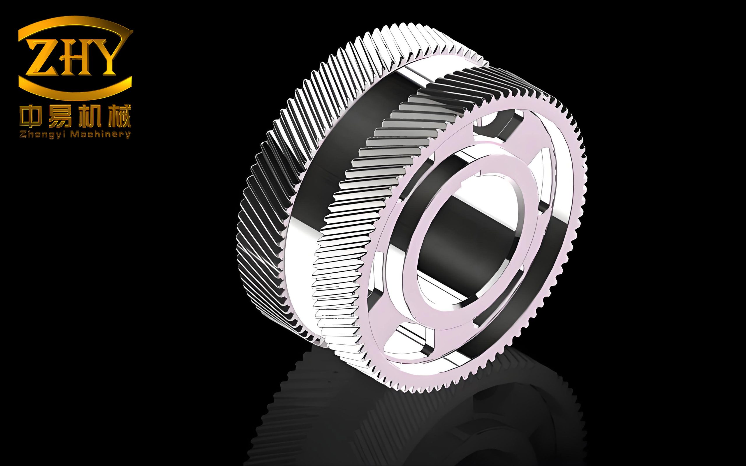
Herringbone gears are widely employed in high-speed, high-load power transmission systems such as aerospace gearboxes and marine propulsion units, owing to their excellent characteristics of high contact ratio, balanced axial forces, and smooth meshing performance. In this work, I focus on the compound modification design and meshing performance analysis of a double helical star gear system used in an advanced geared turbofan engine. The study encompasses low slip ratio parameter optimization, thermoelastic coupling analysis, derivation of compound modification tooth surfaces, accurate computation of time-varying meshing stiffness, and comprehensive dynamic analysis of the gear system. The findings demonstrate that compound modification significantly improves load distribution, reduces meshing impact, and lowers vibration levels, which is of great theoretical significance and engineering value for vibration and noise reduction of high-speed heavy-load herringbone gears.
1. Introduction
With the rapid advancement of machinery toward higher speed, higher efficiency, and heavier loads, the demand for reliable power transmission systems has intensified. Herringbone gears, also known as double helical gears, possess distinct advantages over conventional helical or spur gears. Their symmetrical helix structure cancels out axial thrust forces, allowing for higher power density and smoother operation. These attributes make them particularly suitable for critical applications such as main gearboxes in helicopters, marine propulsion systems, and aero-engine reduction gearboxes. In the context of the geared turbofan (GTF) engine, the star herringbone gear train plays a pivotal role in reducing the engine’s noise footprint while maintaining high efficiency and reliability.
However, high-speed and heavy-load operating conditions introduce significant challenges. During meshing, herringbone gears experience combined effects of elastic deformation under load and thermal deformation due to frictional heating. These deformations, alongside inevitable manufacturing and assembly errors, often lead to meshing interference at tooth entry and exit, stress concentration, uneven load distribution, and amplified vibration and noise. To mitigate these adverse effects, tooth modification has proven to be an effective and economic technique. By deliberately removing material from specific regions of the tooth flank—either along the profile or the lead direction—the geometric mismatch at mesh entry and exit can be minimized, leading to reduced dynamic excitation and improved load sharing among teeth.
This research is dedicated to a comprehensive investigation of compound modification—combining both profile and lead modification—applied to herringbone gears. The objectives are to establish a rigorous design methodology, to quantify its impact on time-varying meshing stiffness, and to evaluate the dynamic behavior of the entire star gear system. The study integrates analytical modeling, numerical simulation, and optimization algorithms to provide both theoretical insight and practical engineering guidelines.
The remainder of this paper is organized as follows. Section 2 details the parameter optimization based on low slip ratio and subsequent thermoelastic coupling analysis. Section 3 presents the derivation of compound modification tooth surfaces and the finite element contact analysis. Section 4 elaborates a novel analytical model for calculating the time-varying meshing stiffness of modified herringbone gears, followed by parametric studies. Section 5 establishes the lumped parameter dynamic model of the star gear system, incorporating friction excitations, mesh phasing, and time-varying stiffness, to evaluate the dynamic performance before and after modification. Section 6 concludes the paper with key findings.
2. Parameter Optimization and Thermoelastic Coupling Analysis
2.1 Slip Ratio Calculation of Herringbone Gear Pairs
Slip ratio, also known as specific sliding, is a critical design parameter that quantifies the relative sliding motion between mating tooth surfaces. A high slip ratio leads to significant frictional heating, surface wear, and reduced transmission efficiency. For herringbone gears, minimizing the maximum slip ratio and balancing the slip ratios between the driving and driven members are essential for improving scuffing resistance and durability.
As illustrated in Figure 2.1 (conceptual diagram), the slip ratio of a gear pair is defined based on the relative tangential velocities of the mating tooth flanks. For the driving gear (gear 1) and driven gear (gear 2), the slip ratios $\eta_1$ and $\eta_2$ at the meshing point K can be expressed as:
$$
\begin{aligned}
\eta_1 &= \frac{|d s_{K1} – d s_{K2}|}{d s_{K1}} = \frac{1+i}{i}\left(1 – \frac{L}{\rho_1}\right) \\
\eta_2 &= \frac{|d s_{K1} – d s_{K2}|}{d s_{K2}} = (1+i)\left(1 – \frac{L}{i \rho_2}\right)
\end{aligned}
$$
where $i$ is the gear ratio, $L$ is the length of the line of action, and $\rho_1$, $\rho_2$ are the instantaneous radii of curvature at the contact point for the two gears. The line of action length $L$ can be computed from the base radii and the operating center distance, and it depends on parameters such as the module $m_t$, the pressure angle $\alpha_t$, the number of teeth $z_1$, $z_2$, and the center distance modification coefficient $y$:
$$
L = m_t \cos\alpha_t \left[ \frac{(z_1 + z_2)}{2} + y \right]
$$
To further investigate the influence of gear parameters on the slip ratio of herringbone gears, I computed the slip ratio distribution along the path of contact for various design scenarios. Table 2.1 summarizes the effect of key design parameters on the slip ratio.
| Parameter (Range) | Effect on Slip Ratio |
|---|---|
| Helix angle $\beta$ (15° to 30°) | Higher $\beta$ significantly reduces slip ratio |
| Normal pressure angle $\alpha_n$ (15° to 25°) | Higher $\alpha_n$ moderately reduces slip ratio |
| Normal module $m_n$ (2 to 12 mm) | Negligible effect on slip ratio |
| Total addendum modification coefficient $\Sigma x$ (-0.2 to 0.4) | Higher $\Sigma x$ reduces slip ratio |
| Gear ratio $u$ (31/37 to 37/31) | Higher $u$ slightly increases slip ratio |
2.2 Optimization of Design Parameters for Low Slip Ratio
To achieve a balanced and minimized slip ratio for the star herringbone gear system, I developed a parameter optimization model. The design variables included the tooth numbers $z_1$, $z_2$, $z_3$ for the sun, planet, and ring gears, the normal module $m_n$, the helix angle $\beta$, the normal pressure angle $\alpha_n$, and the addendum modification coefficients $x_{n1}$, $x_{n2}$, $x_{n3}$. The objective function was to minimize the sum of absolute maximum slip ratios of both the sun-planet and planet-ring meshes:
$$
\min f(\mathbf{X}) = |\eta_{1\max}| + |\eta_{2\max}| + |\eta_{3\max}| + |\eta_{4\max}|
$$
This objective was subjected to a set of constraints including constant gear ratio preservation, center distance tolerance, assembly conditions for five planets, root interference avoidance, tooth tip thickness, and standard value constraints for module and pressure angle. I employed MATLAB’s optimization toolbox, utilizing the fmincon function for global search combined with a branch-and-bound algorithm for discrete variables. The optimized parameters are presented in Table 2.2.
| Parameter | Sun Gear | Planet Gear | Ring Gear |
|---|---|---|---|
| Tooth number $z$ | 44 | 41 | 126 |
| Normal module $m_n$ (mm) | 1.5 | ||
| Normal pressure angle $\alpha_n$ (°) | 25 | ||
| Helix angle $\beta$ (°) | 31.9218 | ||
| Addendum modification coefficient $x_n$ | 0.056 | 0.2077 | 0.47 |
The comparison of maximum slip ratios before and after optimization is presented in Table 2.3. The optimization achieved a substantial reduction in slip ratios for all meshing pairs, with the largest reduction being 53.24% for the planet-ring gear pair.
| Mesh Pair | Before Optimization | After Optimization | Reduction (%) |
|---|---|---|---|
| Sun (drive) – Planet (driven) | 0.6573 | 0.4018 | 38.87% |
| Planet (drive) – Sun (driven) | 0.6573 | 0.3408 | 31.56% |
| Planet (drive) – Ring (driven) | 0.2765 | 0.1293 | 53.24% |
| Ring (drive) – Planet (driven) | 0.1643 | 0.1113 | 31.88% |
2.3 Heat Flux and Convection Coefficient
Under the rated operating condition of 2000 kW input power and 7500 r/min input speed, the frictional heat generated on the tooth surfaces is significant. The heat flux due to friction can be calculated based on Hertzian contact theory and the relative sliding velocity $v_f$:
$$
q_t = \mu_f p_n v_f \varphi
$$
where $q_t$ is the total heat flux, $\mu_f$ is the friction coefficient, $p_n$ is the normal contact pressure, and $\varphi$ is the conversion coefficient of friction work into heat (assumed to be 0.9). The heat flux is distributed between the two meshing gears according to the heat partition ratio $\xi$, which depends on the thermal properties of the gear materials:
$$
\xi_1 = \frac{\sqrt{\lambda_1 \rho_1 c_1 v_{t1}}}{\sqrt{\lambda_1 \rho_1 c_1 v_{t1}} + \sqrt{\lambda_2 \rho_2 c_2 v_{t2}}}
$$
Here, $\lambda$, $\rho$, $c$ are the thermal conductivity, density, and specific heat of the gear material, respectively, and $v_{t1}$, $v_{t2}$ are the tangential velocities of the contact points on the two gears.
Figures 2.7(a)-(h) show the heat flux distribution on the tooth surfaces of the sun gear, planet gear (both meshing sides), and ring gear. The analysis reveals that the heat flux is symmetrically distributed along the tooth width, with significantly higher values near the tooth root and tip, and near-zero values at the pitch point where pure rolling occurs. A direct comparison between the original and optimized designs confirms that the parameter optimization for low slip ratio effectively reduces the heat flux across all gear components, thereby lowering the thermal load on the herringbone gears.
In addition to heat flux, accurate thermal boundary conditions require the calculation of convective heat transfer coefficients on both the end faces and the tooth surfaces of herringbone gears. For the end face (treated as a rotating disc), the convective coefficient $h_r$ depends on the flow regime characterized by the Reynolds number $Re$:
$$
h_r = 0.308 \left( \frac{\omega r^2}{v_f} \right)^{0.5} \lambda_f^{0.5} P_r^{0.33} \quad \text{(laminar)}
$$
$$
h_r = 0.0197 \left( \frac{\omega r^2}{v_r} \right)^{0.8} \lambda_r^{0.6} P_r^{0.6} \quad \text{(turbulent)}
$$
where $\omega$ is the angular velocity, $r$ is the radius, $v_r$ is the kinematic viscosity of the lubricant-air mixture, $k_r$ is the thermal conductivity, and $P_r$ is the Prandtl number. The convective coefficient on the tooth flank for oil-jet lubrication is calculated using:
$$
h_c = \frac{k_0}{b} \sqrt{\frac{\omega_i R_i}{\alpha_0}} \left( \frac{q_{tot} A}{4\pi R_i \omega_i b} \right)^{0.25}
$$
where $k_0$ is the thermal conductivity of the oil, $\alpha_0$ is the thermal diffusivity, $\omega_i$ is the angular velocity of the gear, $R_i$ is the radius at any point on the tooth, $A$ is the tooth surface area, and $b$ is the tooth width. Table 2.4 summarizes the calculated convective heat transfer coefficients.
| Component | Surface | Before | After |
|---|---|---|---|
| Sun gear | End face | 175.96 | 177.84 |
| Sun gear | Tooth flank | 2561.48 | 2069.80 |
| Planet gear | End face | 183.47 | 183.78 |
| Planet gear | Tooth flank (sun side) | 2745.23 | 2182.38 |
| Planet gear | Tooth flank (ring side) | 2746.19 | 2178.58 |
| Ring gear | End face | 107.81 | 107.49 |
| Ring gear | Tooth flank | 1176.38 | 938.61 |
2.4 Temperature Field and Thermoelastic Coupling Analysis
Using the calculated thermal boundary conditions, I established finite element models of the complete star herringbone gear system in ANSYS. The SOLID70 thermal element was used for mesh discretization, with a total of approximately 6.21 million elements and 6.47 million nodes for the original model, and 10.04 million elements and 10.4 million nodes for the optimized model. Figure 2.10 and Figure 2.11 present the steady-state temperature contours of the sun gear, planet gear, ring gear, and the full system. Table 2.5 summarizes the key temperature values.
| Component | Before Optimization | After Optimization | ||
|---|---|---|---|---|
| Max. Temp. | Max. Rise | Max. Temp. | Max. Rise | |
| Sun gear | 140.577 | 80.577 | 115.063 | 55.063 |
| Planet gear | 86.710 | 26.710 | 78.415 | 18.415 |
| Ring gear | 102.222 | 42.222 | 89.745 | 29.745 |
The results demonstrate a significant decrease in temperature rise for all gear components after the low-slip-ratio parameter optimization. The sun gear experiences the highest temperature reduction of 25.49°C in the maximum temperature rise, followed by the ring gear (12.48°C) and the planet gear (8.30°C). This confirms that minimizing the slip ratio of herringbone gears is an effective strategy to reduce frictional heat generation in high-speed applications.
To assess the combined effects of thermal and mechanical loading, I performed a thermoelastic coupling analysis. The SOLID70 thermal elements were converted to SOLID45 structural elements, and the temperature field was applied as a body load. The mechanical boundary conditions included constraining the sun gear’s inner bore in the axial and radial directions while applying torque in the tangential direction, constraining the planet gear’s inner bore, fully constraining the ring gear’s outer surface, and establishing contact pairs at the meshing tooth interfaces. Figure 2.13 shows the total displacement contours at the meshing-in and meshing-out positions for the optimized herringbone gear pair.
The thermoelastic coupling analysis reveals the interference patterns at critical meshing positions. At the meshing-in position, the sun gear tooth root and the planet gear tooth tip exhibit significant mutual interference. Conversely, at the meshing-out position, the sun gear tooth tip and the planet gear tooth root interfere. These interferences are quantified by extracting the displacements along the line of action at the meshing points and adjacent contact points, as listed in Table 2.6. These data form the basis for calculating the profile modification parameters in Section 3.
| Measurement Point | Sun Gear | Planet Gear |
|---|---|---|
| Mesh-in point displacement $\delta_{ei}$ | 36.81 | 58.20 |
| Mesh-out point displacement $\delta’_{ei}$ | 57.06 | 37.54 |
| Adjacent tooth contact point displacement $\delta_c$ (mesh-in) | 27.38 | |
| Adjacent tooth contact point displacement $\delta’_c$ (mesh-out) | 28.39 | |
3. Compound Modification Design
3.1 Modification Parameter Calculation
Based on the thermoelastic coupling analysis results, I calculated the compound modification parameters—lead modification and profile modification—for the sun gear and planet gear of the herringbone gear set. The ring gear is generally not modified due to manufacturing complexity and its internal gear geometry.
For the lead modification amount, considering the thermal expansion of the gear body under operating conditions, the modification amount $\Delta\delta$ is determined by:
$$
\Delta\delta = 0.5 \xi_r \lambda_r r \left[ \left(t_{sh} – t_{ch}\right) – \left(t_{s1} – t_{c1}\right) \right] \sin\alpha_t
$$
where $\xi_r$ is the coefficient of linear expansion, $\lambda_r$ is the thermal deformation correction factor (taken as 0.75), $r$ is the pitch circle radius, $t_{sh}$ and $t_{ch}$ are the maximum outer surface and bore temperatures, respectively, and $t_{s1}$ and $t_{c1}$ are the minimum outer surface and bore temperatures. Using the temperature data from the thermoelastic analysis, I obtained lead modification amounts of 10.083 μm for the sun gear and 9.796 μm for the planet gear. For manufacturing convenience, a common value of 10 μm was adopted for both gears.
The profile modification parameters include the modification amount and the modification length at both the tooth tip and tooth root. The modification length $h$ is determined by the base pitch and the transverse contact ratio $\varepsilon_\alpha$:
$$
h = \frac{p_{bt}}{2}(\varepsilon_\alpha – 1)
$$
where $p_{bt}$ is the transverse base pitch. The modification amount at the mesh-in and mesh-out positions is derived from the tooth deformation interference. The normal backlash change $\Delta f$ is calculated from the relative displacements of the meshing teeth:
$$
\Delta f = \left[ \delta_{ei} \left(\cos\theta_{ei}\right) – \delta_{c} \left(\cos\theta_{c}\right) \right] – \left[ \delta’_{ei} \left(\cos\theta’_{ei}\right) – \delta’_{c} \left(\cos\theta’_{c}\right) \right]
$$
Table 3.1 compares the profile modification amounts obtained from the simulation with two classical empirical formulas (KISSsoft and H. Sigg). The agreement is good, confirming that the thermoelastic-coupling-based method is reliable. Since the computed tip and root modification amounts are nearly equal (approximately 10 μm), symmetric profile modification (equal amounts at tip and root) was adopted.
| Method | Sun Gear | Planet Gear |
|---|---|---|
| Simulation (Thermoelastic) | 9.94 (tip) / 9.88 (root) | 9.88 (tip) / 9.94 (root) |
| KISSsoft calculation | 10 / 10 | 10 / 10 |
| H. Sigg formula | 8.39 / 10.6 | 10.6 / 8.39 |
The final compound modification parameters for the sun and planet herringbone gears are summarized in Table 3.2.
| Parameter | Sun Gear | Planet Gear |
|---|---|---|
| Lead modification amount (μm) | 10 | |
| Lead modification length (mm) | 12 | |
| Tip profile modification amount (μm) | 10 | |
| Root profile modification amount (μm) | 10 | |
| Tip profile modification length (mm) | 0.46 | |
| Root profile modification length (mm) | 0.46 | |
3.2 Derivation of Compound Modification Tooth Surface Equation
To accurately model the modified herringbone gears, I derived the mathematical equation of the tooth surface using the theory of gearing. The manufacturing process is simulated using a hypothetical rack cutter whose cutting edge is modified. The rack cutter’s transverse profile is composed of four segments: the involute generating straight line (CD), a parabolic curve for the tip modification (DE), a parabolic curve for the root modification (BC), and an elliptical arc for the root fillet (AB).
The coordinate system of the hypothetical rack cutter is shown in Figure 3.4. The tip modification curve is expressed in its local coordinate system $S_a(x_a O_a y_a)$ as:
$$
\mathbf{R}_a^{(2)} = \begin{bmatrix} u_1 \\ -a_{1} u_1^{n} \end{bmatrix}
$$
Similarly, the root modification curve in local system $S_b(x_b O_b y_b)$ is:
$$
\mathbf{R}_b^{(3)} = \begin{bmatrix} u_2 \\ -a_{2} u_2^{n} \end{bmatrix}
$$
where $a_1$, $a_2$ are the coefficients of the parabolic modification curves, and $n$ is the modification curve order. These local coordinates are transformed to the rack cutter coordinate system $S_0(x_0 O y_0)$ using homogeneous transformation matrices:
$$
\mathbf{R}_0^{(2)} = \mathbf{M}_{0a} \mathbf{R}_a^{(2)}, \quad \mathbf{R}_0^{(3)} = \mathbf{M}_{0b} \mathbf{R}_b^{(3)}
$$
where the transformation matrices $\mathbf{M}_{0a}$, $\mathbf{M}_{0b}$ involve the coordinates of points D and C, respectively. The orientation of the cutters in $S_0$ is:
$$
\mathbf{M}_{0a} = \begin{bmatrix} \cos\alpha_t & -\sin\alpha_t & 0 & x_D \\ \sin\alpha_t & \cos\alpha_t & 0 & y_D \\ 0 & 0 & 1 & 0 \\ 0 & 0 & 0 & 1 \end{bmatrix}
$$
Next, the rack cutter coordinates are transformed to the gear blank coordinate system $S_1(x_1 O_1 y_1)$. For the right-hand helical flank, the transformation is:
$$
\mathbf{M}_{10} = \begin{bmatrix} 1 & 0 & 0 & 0 \\ 0 & 1 & 0 & -\cos\beta \\ 0 & 0 & 1 & -\sin\beta \\ 0 & 0 & 0 & 1 \end{bmatrix}
$$
where $\beta$ is the helix angle. The meshing condition between the rack cutter and the gear blank is determined by the equation of gearing:
$$
\mathbf{n} \cdot \mathbf{v} = 0
$$
This condition leads to a relationship between the rack cutter displacement $l_z$ and the gear rotation angle $\varphi_i$:
$$
\varphi_i = \frac{n_{ix} R_{iy} – n_{iy} R_{ix}}{r n_{ix}}
$$
Finally, the tooth surface of the gear is obtained in the gear coordinate system $S_2(x_2 O_2 y_2)$ via the transformation:
$$
\mathbf{R}_2 = \mathbf{M}_{21} \mathbf{R}_1
$$
with the rotation matrix:
$$
\mathbf{M}_{21} = \begin{bmatrix} \cos\varphi_i & \sin\varphi_i & 0 & -r(\cos\varphi_i + \varphi_i \sin\varphi_i) \\ -\sin\varphi_i & \cos\varphi_i & 0 & -r(\sin\varphi_i – \varphi_i \cos\varphi_i) \\ 0 & 0 & 1 & 0 \\ 0 & 0 & 0 & 1 \end{bmatrix}
$$
To implement the lead modification, I considered the relative motion between the grinding wheel and the gear during the grinding process. The radial infeed of the grinding wheel $C_C$ is controlled as a function of the axial position $z$ to generate the desired lead modification. For a circular arc lead modification:
$$
C_C(z) = r_C – \sqrt{r_C^2 – l_z^2}
$$
for $0 \le z \le l$, where $r_C$ is the radius of the circular arc defined by the lead modification amount and length:
$$
r_C = \frac{l^2 + C^2}{2C}
$$
For a parabolic lead modification of order $n$:
$$
C_C(z) = a_3 l_z^{n}
$$
where $a_3 = C / l^{n}$. By combining the profile modification tooth surface with the lead modification motion path, the final compound modified tooth surface equation of herringbone gears is derived as:
$$
\mathbf{R}_3 = \mathbf{M}_{3a} \mathbf{M}_{at} \mathbf{R}_2
$$
In matrix form, the final coordinates are expressed as:
$$
\begin{aligned}
x_3 &= x_2 \cos\theta – y_2 \sin\theta + C_C \cos\theta \\
y_3 &= x_2 \sin\theta + y_2 \cos\theta + C_C \sin\theta \\
z_3 &= z_2 + l_z
\end{aligned}
$$
where $\theta$ is the gear rotation angle corresponding to the axial position, $l_z$ is the axial feed of the grinding wheel, and $C_C$ is the radial infeed for lead modification.
3.3 Finite Element Contact Analysis
Based on the derived tooth surface equation, I developed an APDL (ANSYS Parametric Design Language) command script to automatically generate the parameterized solid model of the compound-modified herringbone gear pair. The gear material has an elastic modulus of $E = 2.06 \times 10^{11}$ Pa and a Poisson’s ratio of $\mu = 0.27$. The rated operating condition is 400 kW input power at 7500 r/min. The finite element model, as shown in Figure 3.7, was discretized with 1,476,617 elements and 2,560,305 nodes, with local mesh refinement in the tooth contact regions.
Figures 3.8 and 3.9 present the contact stress contours for the sun-planet and planet-ring gear pairs, respectively, before and after compound modification. The analysis yields the following key findings:
- The unmodified sun-planet gear pair exhibits four pairs of teeth in contact at the specific meshing position, while the compound-modified pair has only three tooth pairs in contact. This indicates that the actual contact ratio of herringbone gears decreases after modification.
- The compound modification significantly reduces the contact area on the tooth surface and eliminates the edge stress concentration observed in the unmodified gear.
- The maximum contact stress of the sun-planet gear pair decreases from 1010.84 MPa (unmodified) to 894.73 MPa (modified), a reduction of 11.5%.
- For the planet-ring gear pair, the maximum contact stress decreases from 474.15 MPa to 417.42 MPa, a reduction of 11.9%.
These results clearly demonstrate that compound modification not only reduces the peak stress but also homogenizes the stress distribution across the tooth surface of herringbone gears, thereby improving the contact performance and load-carrying capacity.
4. Time-Varying Meshing Stiffness Calculation
4.1 Analytical Model for Meshing Stiffness of Modified Herringbone Gears
The time-varying meshing stiffness (TVMS) is a key internal dynamic excitation in gear systems. I have developed an analytical model to compute the TVMS of compound-modified herringbone gears, incorporating the effects of profile modification, lead modification, run-out groove width, and load sharing. The model is based on the potential energy method combined with a slicing technique.
Herringbone gears consist of two opposite-handed helical gears separated by a run-out groove. The total meshing stiffness is decomposed into the transverse (end-face) component and the axial component. The total strain energy stored in the gear mesh system is:
$$
\frac{F^2}{2k} = \sum_{j=1}^{2} \left[ \frac{F^2}{2k_{tb,j}} + \frac{F^2}{2k_{ts,j}} + \frac{F^2}{2k_{ta,j}} + \frac{F^2}{2k_{tf,j}} + \frac{F^2}{2k_{ab,j}} + \frac{F^2}{2k_{at,j}} + \frac{F^2}{2k_{af,j}} \right] + \frac{F^2}{2k_h}
$$
where the subscripts $t$ and $a$ denote transverse and axial components, $b$, $s$, $a$, $f$, $h$ denote bending, shear, compression, foundation, and Hertzian contact, respectively. The single tooth pair mesh stiffness is:
$$
\frac{1}{k} = \sum_{j=1}^{2} \left( \frac{1}{k_{tb,j}} + \frac{1}{k_{ts,j}} + \frac{1}{k_{ta,j}} + \frac{1}{k_{tf,j}} + \frac{1}{k_{ab,j}} + \frac{1}{k_{at,j}} + \frac{1}{k_{af,j}} \right) + \frac{1}{k_h}
$$
The transverse stiffness components are calculated using the slicing technique. Each gear tooth is sliced into thin segments along the tooth width direction. For each slice of thickness $\Delta z$, the bending, shear, and compression stiffness contributions are:
$$
k_{tb} = \sum_{i=1}^{N} \left[ \int_{-x_1}^{x_M} \frac{3(\cos\beta \cos\alpha_z)^2 x^2}{E \Delta z y_x^3} dx \right]^{-1}
$$
$$
k_{ts} = \sum_{i=1}^{N} \left[ \int_{-x_1}^{x_M} \frac{1.2(\cos\beta \cos\alpha_z)^2}{G \Delta z y_x} dx \right]^{-1}
$$
$$
k_{ta} = \sum_{i=1}^{N} \left[ \int_{-x_1}^{x_M} \frac{(\cos\beta \sin\alpha_z)^2}{2 E \Delta z y_x} dx \right]^{-1}
$$
where $N$ is the total number of slices, $\Delta z = (2B + B_t)/N$ is the slice thickness, $B$ is the width of one helical half, $B_t$ is the run-out groove width, $\alpha_z$ is the local transverse pressure angle, and $y_x$ is the half-tooth thickness at distance $x$ from the tooth root. The coordinate $x$ varies from $x_1$ (at the tooth root) to $x_M$ (at the load application point).
The Hertzian contact stiffness is expressed as:
$$
k_h = \frac{\pi E L}{4(1-\mu^2)}
$$
where $L$ is the total contact line length. The gear foundation transverse stiffness is approached using the analytical formula by Sainsot et al.:
$$
k_{tf} = \sum_{i=1}^{N} \frac{E \Delta z}{\cos^2\beta \cos^2\alpha_z} \left[ \frac{L^*}{2} \left( \frac{u_f}{S_f} \right)^2 + M^* \left( \frac{u_f}{S_f} \right) + P^* (1 + Q^* \tan^2\alpha_z) \right]
$$
where $L^*$, $M^*$, $P^*$, $Q^*$ are coefficients depending on $u_f$ and $S_f$ (geometric parameters of the tooth root circle).
For the axial direction, the axial bending and axial torsional stiffness components are derived considering the axial force component acting on the helical teeth:
$$
k_{ab} = \sum_{i=1}^{N} \left[ \int_{-x_1}^{x_M} \frac{\sin^2\beta \cos^2\alpha_z \left( \frac{1}{N_s}\sum_{s=1}^{N_s} x – x \right)^2}{E I_{ax}} dx \right]^{-1}
$$
$$
k_{at} = \sum_{i=1}^{N} \left[ \int_{-x_1}^{x_M} \frac{\sin^2\beta \cos^2\alpha_z \left( \frac{1}{N_s}\sum_{s=1}^{N_s} y \right)^2}{G I_p} dx \right]^{-1}
$$
The foundation axial stiffness considers the bending deformation of the gear body including the run-out groove:
$$
k_{af} = \left[ \int_{r_0}^{r_f} \frac{\sin^2\beta \cos^2\alpha_z \left( \frac{1}{N_s}\sum_{s=1}^{N_s} x_s – x \right)^2}{E I_{af}} dx \right]^{-1}
$$
where $r_0$ is the bore radius, $r_f$ is the root circle radius, and $I_{af}$ is the area moment of inertia of the gear body cross-section, which depends on the gear body dimensions including the run-out groove radius. The axial area moment of inertia is formulated as:
$$
I_{af} = \begin{cases}
\frac{1}{3} B \left( r_f^2 – r_0^2 \right) \left( r_f^2 – x^2 \right) + \frac{2}{3} \left( r_f^3 – r_0^3 \right) & r_0 \le x \le r_t \\
\frac{1}{3} B \left( r_f^2 – r_t^2 \right) \left( r_f^2 – x^2 \right) + \frac{1}{3} B_t \left( r_t^2 – x^2 \right)^2 & r_t \le x \le r_f
\end{cases}
$$
4.2 Mesh Contact State of Modified Herringbone Gears
To accurately capture the meshing behavior of modified herringbone gears, I accounted for the variation of the actual contact start and end points caused by profile modification and load-induced deformation. Under an applied load $F$, the tooth deformation $\delta$ of each meshing pair is:
$$
\delta(\alpha_z) = \frac{F}{k(\alpha_z)}
$$
where $k(\alpha_z)$ is the instantaneous single-pair mesh stiffness. Since the total deformation is the same for all pairs in simultaneous mesh, the load distribution is determined by their respective stiffness values.
Based on the geometric deviation $\Delta(\alpha_z)$ of the modified tooth profile relative to the theoretical involute, I developed a numerical procedure to determine the actual mesh start and end points. The modified tooth profile is discretized along its height, and the point where the geometrical deviation exceeds the total deformation is identified as the point where contact commences or terminates. This calculation yields the actual effective line of action length, and consequently, the actual contact ratio of herringbone gears.
For the gear pair under study, the analytical results yield the following mesh start and end radii: $r’_{s1} = 37.731$ mm and $r’_{e1} = 41.093$ mm. This is compared against the finite element value obtained from the contact simulation: 38.004 mm and 41.226 mm, respectively. The discrepancies are merely 0.72% and 0.32%, confirming the accuracy of the analytical approach.
The total contact ratio of the modified herringbone gear pair is decomposed into the transverse contact ratio $\varepsilon’_\alpha$ and the overlap (axial) contact ratio $\varepsilon’_\beta$:
$$
\varepsilon’_\alpha = \frac{\sqrt{r’^2_{e1} – r^2_{b1}} + \sqrt{r’^2_{e2} – r^2_{b2}} – (r_{b1} + r_{b2})\tan\alpha’_{wt}}{p_{bt}}
$$
$$
\varepsilon’_\beta = \frac{B’ \sin\beta}{\pi m_n}
$$
where $r’_{e1}$, $r’_{e2}$ are the radii to the actual mesh start/end points, $r_b$ is the base circle radius, $p_{bt}$ is the transverse base pitch, $\alpha’_{wt}$ is the operating pressure angle, and $B’$ is the effective tooth width considering the lead modification. Using this method, I validated the computed total contact ratio against the finite element predictions, as shown in Figure 4.6, where the tooth contact state is clearly visualized.
The time-varying contact line length $L(t)$ is a critical parameter for the stiffness calculation. Considering the actual contact ratio and lead modification, the contact line length varies with time as shown in Figure 4.8, where the analytical stiffness curve is compared with the FEM result. The average stiffness computed from the analytical method is $8.134 \times 10^8$ N/m, while the FEM result is $8.361 \times 10^8$ N/m, yielding an error of only 2.71%, which is well within the engineering acceptance range.
4.3 Parametric Study of Meshing Stiffness
Using the validated analytical model, I conducted a series of parametric studies to investigate the effects of various factors on the TVMS of herringbone gears. The baseline gear parameters are listed in Table 4.1.
| Parameter | Symbol | Value |
|---|---|---|
| Number of teeth (sun/planet) | $Z_1$ / $Z_2$ | 44 / 41 |
| Normal module (mm) | $m_n$ | 1.5 |
| Normal pressure angle (°) | $\alpha_n$ | 25 |
| Helix angle (°) | $\beta$ | 31.9218 |
| Tooth width (one half) (mm) | $B$ | 24 |
| Run-out groove width (mm) | $B_t$ | 10 |
| Center distance (mm) | $a$ | 75.5 |
| Input speed (r/min) | $n$ | 7500 |
| Input torque (N·m) | $T$ | 510 |
| Elastic modulus (Pa) | $E$ | $2.1 \times 10^{11}$ |
4.3.1 Effect of Run-out Groove Width
I examined the influence of the run-out groove width $B_t$ (ranging from 0 to 40 mm) on the meshing stiffness of herringbone gears, while keeping the tooth width constant. The results, shown in Table 4.2 and Figure 4.9, indicate that a wider run-out groove increases the gear body stiffness, thereby increasing the overall meshing stiffness. The fluctuation amplitude remains nearly unchanged because the contact ratio is unaffected by the groove width.
| $B_t$ (mm) | $\varepsilon’_\alpha$ | $\varepsilon’_\beta$ | Mean $k$ (×10⁸ N/m) | Fluctuation (×10⁸ N/m) |
|---|---|---|---|---|
| 0 | 0.970 | 2.693 | 8.248 | 0.332 |
| 10 | 0.970 | 2.693 | 8.349 | 0.333 |
| 20 | 0.970 | 2.693 | 8.482 | 0.330 |
| 30 | 0.970 | 2.693 | 8.624 | 0.328 |
| 40 | 0.970 | 2.693 | 8.793 | 0.327 |
4.3.2 Effect of Profile Modification Parameters
I first investigated the effect of the profile modification amount $\Delta g$ on the meshing stiffness. The modification amount was varied from 0 to 14 μm, and the results are presented in Table 4.3 and Figure 4.10. Key observations include:
- The contact ratio decreases with increasing modification amount due to the reduced effective tooth height.
- The mean meshing stiffness decreases as the modification amount increases.
- The stiffness fluctuation exhibits a non-monotonic behavior; it initially decreases and then increases. The optimal modification amount for minimizing fluctuation is approximately 10 μm, which corresponds to the case where the actual transverse contact ratio is closest to an integer value.
| $\Delta g$ (μm) | $\varepsilon’_\alpha$ | Total $\varepsilon$ | Mean $k$ (×10⁸ N/m) | Fluctuation (×10⁸ N/m) |
|---|---|---|---|---|
| 0 (unmodified) | 1.203 | 3.896 | 10.392 | 0.543 |
| 8 | 1.126 | 3.819 | 9.420 | 0.256 |
| 10 | 1.048 | 3.741 | 8.673 | 0.238 |
| 12.5 | 0.970 | 3.663 | 8.134 | 0.342 |
| 14 | 0.893 | 3.586 | 7.842 | 0.398 |
Next, I examined the effect of the profile modification length $h_g$ and the modification curve order $n$. The results are illustrated in Tables 4.4 and 4.5 and Figures 4.11 and 4.12. Similar to the modification amount, increasing the modification length reduces the contact ratio and mean stiffness. The modification curve order also significantly impacts the stiffness: lower-order curves (e.g., linear, $n=1$) remove more material and thus reduce the stiffness more dramatically. The third-order curve ($n=3$) yields the smallest stiffness fluctuation for the herringbone gear pair.
| $h_g$ (mm) | $\varepsilon’_\alpha$ | Total $\varepsilon$ | Mean $k$ (×10⁸ N/m) | Fluctuation (×10⁸ N/m) |
|---|---|---|---|---|
| 0.6 | 1.048 | 3.741 | 9.373 | 0.204 |
| 0.8 | 0.981 | 3.674 | 8.588 | 0.215 |
| 1.0 | 0.970 | 3.663 | 8.134 | 0.342 |
| 1.2 | 0.893 | 3.586 | 7.675 | 0.478 |
| Curve Order $n$ | $\varepsilon’_\alpha$ | Total $\varepsilon$ | Mean $k$ (×10⁸ N/m) | Fluctuation (×10⁸ N/m) |
|---|---|---|---|---|
| 1 (linear) | 0.738 | 3.431 | 6.561 | 0.874 |
| 2 | 0.970 | 3.663 | 8.140 | 0.349 |
| 3 | 1.028 | 3.721 | 8.805 | 0.178 |
| 4 | 1.048 | 3.741 | 9.165 | 0.234 |
| 6 | 1.126 | 3.819 | 9.546 | 0.319 |
4.3.3 Effect of Lead Modification
For the lead modification of herringbone gears, I analyzed the influence of the modification amount, length, and curve order. Table 4.6 and Figure 4.13 demonstrate that an increase in the lead modification amount reduces the effective tooth width, decreasing the overlap ratio and the mean meshing stiffness. A lead modification amount of 10 μm yields the smallest stiffness fluctuation, corresponding to an axial contact ratio very close to an integer (2.074).
| $\Delta g$ (μm) | $\varepsilon’_\beta$ | Total $\varepsilon$ | Mean $k$ (×10⁸ N/m) | Fluctuation (×10⁸ N/m) |
|---|---|---|---|---|
| 0 (unmodified) | 2.693 | 3.896 | 10.392 | 0.543 |
| 6 | 2.693 | 3.896 | 10.389 | 0.543 |
| 7 | 2.505 | 3.708 | 9.749 | 0.643 |
| 8 | 2.343 | 3.546 | 8.978 | 0.504 |
| 10 | 2.074 | 3.277 | 8.169 | 0.126 |
| 12 | 1.912 | 3.115 | 7.559 | 0.360 |
Tables 4.7 and 4.8 list the effects of the lead modification length and curve order. In summary, the lead modification length and curve order affect the meshing stiffness of herringbone gears in a manner analogous to the profile modification parameters, with the primary mechanism being the reduction of the effective tooth width.
| $h_g$ (mm) | $\varepsilon’_\beta$ | Total $\varepsilon$ | Mean $k$ (×10⁸ N/m) | Fluctuation (×10⁸ N/m) |
|---|---|---|---|---|
| 3 | 2.612 | 3.816 | 10.116 | 0.621 |
| 6 | 2.505 | 3.708 | 9.755 | 0.665 |
| 9 | 2.397 | 3.600 | 9.356 | 0.579 |
| 12 | 2.343 | 3.546 | 8.978 | 0.504 |
| Curve Order $n$ | $\varepsilon’_\beta$ | Total $\varepsilon$ | Mean $k$ (×10⁸ N/m) | Fluctuation (×10⁸ N/m) |
|---|---|---|---|---|
| 1 (linear) | 2.020 | 3.223 | 7.999 | 0.150 |
| 2 | 2.343 | 3.546 | 8.978 | 0.504 |
| 3 | 2.451 | 3.654 | 9.513 | 0.524 |
| 4 | 2.505 | 3.708 | 9.694 | 0.489 |
| 6 | 2.558 | 3.762 | 9.873 | 0.493 |
4.3.4 Effect of Input Torque
Finally, I investigated the effect of the input torque on the meshing stiffness of modified herringbone gears, as presented in Table 4.9 and Figure 4.16. As the input torque increases from 200 to 600 N·m, the tooth deformation increases, causing more of the modified region to participate in meshing, which increases the effective contact ratio and hence the mean meshing stiffness. Table 4.9 shows that the stiffness values increase with torque until the modification regions are fully engaged; beyond this point (at approximately 700 N·m), the stiffness no longer changes significantly.
| Torque (N·m) | $\varepsilon’_\alpha$ | Total $\varepsilon$ | Mean $k$ (×10⁸ N/m) | Fluctuation (×10⁸ N/m) |
|---|---|---|---|---|
| 200 | 0.893 | 3.586 | 7.595 | 0.467 |
| 300 | 0.990 | 3.683 | 8.495 | 0.221 |
| 400 | 1.048 | 3.741 | 9.331 | 0.240 |
| 500 | 1.126 | 3.819 | 10.039 | 0.452 |
| 600 | 1.203 | 3.896 | 10.384 | 0.564 |
| 700 | 1.203 | 3.896 | 10.385 | 0.561 |
5. Dynamic Characteristics Analysis
5.1 Tooth Surface Load, Friction Force, and Friction Torque Distribution
To evaluate the dynamic performance of the star herringbone gear system, I first determined the load distribution on the tooth surface of the herringbone gears. Based on the time-varying meshing stiffness calculated in Section 4 and the slicing approach, the normal load on each tooth slice is calculated by:
$$
F_i = \frac{k_i}{\sum_{i=1}^{N_c} k_i} F
$$
where $F$ is the total transmitted load, $k_i$ is the instantaneous stiffness of tooth slice $i$, and $N_c$ is the number of slices in contact. Figure 5.1 shows the normal load distribution on the sun gear tooth surface under different modification scenarios: (a) unmodified, (b) profile modified, (c) lead modified, and (d) compound modified.
The analysis yields the following insights:
- The load distribution of herringbone gears is symmetric on the left and right helical halves.
- The unmodified gear tooth exhibits the largest loaded area, whereas the compound-modified herringbone gear tooth has a considerably reduced loaded region in both the tooth height and width directions.
- The profile-modified gear primarily reduces the loaded area along the tooth height, while the lead-modified gear reduces it along the tooth width.
- Since the total transmitted load is constant, a smaller loaded area results in a higher unit load. Nevertheless, the compound modification homogenizes the load distribution and eliminates edge concentration effects, which is beneficial for the gear’s load-carrying capacity.
Over-modification can lead to an elliptical load distribution with a significant reduction of the loaded area, as shown in Figure 5.2, which substantially increases the unit load and reduces the load-carrying capacity of herringbone gears. Therefore, precise control of the modification amount is crucial in manufacturing.
Following the Coulomb friction law, the friction force $f(t)$ and friction torque $T_f(t)$ on the tooth surface of herringbone gears are calculated as:
$$
f(t) = \mu(t) F(t) \cdot \text{sign}(M)
$$
$$
T_f(t) = f(t) r_b
$$
where $\mu(t)$ is the friction coefficient (taken as a constant average value of 0.05 in this study), $F(t)$ is the dynamic meshing force, sign($M$) determines the direction based on the relative sliding direction with respect to the pitch point, and $r_b$ is the base circle radius.
Figures 5.4 and 5.5 illustrate the friction force and friction torque of the sun gear for the four modification scenarios. Consistent with the load distribution results, the friction force and torque on herringbone gears are symmetrically distributed along the tooth width direction. Since the modified gear tooth has a smaller loaded area, the unit load is higher, leading to marginally higher friction force and friction torque on the modified gear surfaces. This is an inherent trade-off of tooth modification, but the resulting vibrational benefits far outweigh this drawback, as shown below.
5.2 Mesh Phasing Analysis of the Star Herringbone Gear System
In the star herringbone gear system, five planet gears mesh simultaneously with the central sun gear and the internal ring gear. Due to the geometrical arrangement, each sun-planet mesh pair and each planet-ring mesh pair has a distinct meshing phase. These phase differences significantly influence the dynamic response of the system. I therefore conducted a systematic mesh phasing analysis based on the gear geometry.
For the sun gear-planet gear $i$ with respect to sun gear-planet gear 1, the mesh phase difference $\Delta t_{i}$ is:
$$
\Delta t_i = T \cdot \text{mod} \left[ \frac{2\sqrt{r_{bs}^2 + r_{bp}^2} + 2(i-1)r_{bs}\frac{2\pi}{5}}{p_{bt}} – \frac{\sqrt{r_{ap}^2 – r_{bp}^2} + \sqrt{r_{as}^2 – r_{bs}^2}}{p_{bt}} \right]
$$
Similarly, the phase difference between the sun gear-planet gear 1 mesh and the planet gear $i$-ring gear mesh is calculated based on the geometry of the internal and external meshing lines:
$$
\Delta t’_i = T \cdot \text{mod} \left[ \frac{\sqrt{r_{ap}^2 – r_{bp}^2} + r_{bp}(\pi + \varphi_i – \psi_i) + \sqrt{r_{ar}^2 – r_{br}^2} + r_{br}\varphi_i}{p_{bt}} \right]
$$
Table 5.1 lists the computed mesh phase differences for all five planet branches, taking the sun gear-planet 1 mesh as the reference.
| Branch $i$ | Sun-Planet Phase Lag $\Delta T_{i1}$ | Planet-Ring Phase Lag $\Delta T_{i2}$ |
|---|---|---|
| 1 | 0.000 | 0.248 |
| 2 | 0.527 | 0.775 |
| 3 | 0.211 | 0.459 |
| 4 | 0.739 | 0.987 |
| 5 | 0.423 | 0.671 |
These phase differences are normalized by the mesh period $T$. Figure 5.8 shows the meshing stiffness curves of all internal and external gear pairs after incorporating the mesh phasing. It is evident that the peak stiffness values of the individual gear pairs occur at different time instants, which helps to smooth out the total system excitation.
5.3 Lumped Parameter Dynamic Model
To investigate the dynamic behavior of the star herringbone gear system, I established a lumped parameter dynamic model with 28 degrees of freedom (DOFs). Each gear (sun gear, five planet gears, ring gear) has four DOFs: two transverse displacements ($x$, $y$), one axial displacement ($z$), and one torsional rotation ($\theta$). The system model is shown in Figure 5.9.
The time-varying meshing stiffness obtained from Section 4 was expanded into a Fourier series:
$$
k(t) = a_0 + \sum_{n=1}^{\infty} \left[ a_n \cos(n\omega_m t) + b_n \sin(n\omega_m t) \right]
$$
where $\omega_m$ is the mesh frequency, given by $\omega_m = 2\pi n_s Z_s / 60$, with $n_s$ being the sun gear speed in r/min and $Z_s$ the sun gear tooth number. The static transmission error $e(t)$ is modeled as a superposition of harmonic functions at the shaft rotation frequency and its harmonics:
$$
e(t) = 0.5 F_p \sin(\omega_f t + \psi_f) + 0.5 f’_t \sin(\omega_m t + \psi_m)
$$
where $F_p$ is the cumulative pitch deviation, $f’_t$ is the single-tooth tangential tolerance, $\omega_f$ is the shaft rotational frequency, and $\psi_f$, $\psi_m$ are phase angles.
The relative displacement of the two gears along the line of action for the $i$-th sun-planet mesh is:
$$
\delta_{w,i} = (x_s – x_{p,i}) \sin\psi_i \cos\beta + (y_s – y_{p,i}) \cos\psi_i \cos\beta + (z_s – z_{p,i}) \sin\beta + r_{bs}\theta_s + r_{bp}\theta_{p,i} – e_{w,i}(t)
$$
For the $i$-th planet-ring mesh, the relative displacement is:
$$
\delta_{n,i} = (x_{p,i} – x_r) \sin\varphi_i \cos\beta + (y_{p,i} – y_r) \cos\varphi_i \cos\beta + (z_{p,i} – z_r) \sin\beta + r_{bp}\theta_{p,i} + r_{br}\theta_r – e_{n,i}(t)
$$
The dynamic meshing force for each gear pair is calculated as:
$$
F_{w,i} = k_{w,i}(\delta_{w,i}) + c_{w,i}(\dot{\delta}_{w,i}) + F_{cw} \varepsilon(m)
$$
$$
F_{n,i} = k_{n,i}(\delta_{n,i}) + c_{n,i}(\dot{\delta}_{n,i}) + F_{cn} \varepsilon(m)
$$
where $c_{w,i}$, $c_{n,i}$ are the mesh damping coefficients, $F_{cw}$, $F_{cn}$ are the mesh-in impact forces, and $\varepsilon(m)$ is a pulse function that activates at the mesh-in instant. The mesh-in impact force is calculated based on the impact velocity $\Delta v$ and the combined compliance of the gear pair:
$$
F_{cw} = \frac{B_s J_s}{J_s / r_{bs}^2 + J_p / r_{bp}^2} \cdot \frac{\Delta v_{sp}}{q_{sw}}
$$
The dynamic equations of motion for the sun gear, planet gears, and ring gear are given in equation sets (5.23) – (5.25). As a representative example, the equations for the sun gear are:
$$
m_s \ddot{x}_s + c_{sx}\dot{x}_s + k_{sx}x_s = \sum_{i=1}^{5} (F_{w,i} \sin\psi_i \cos\beta) + \sum_{i=1}^{5} f_{w,i} \sin\psi_i
$$
$$
m_s \ddot{y}_s + c_{sy}\dot{y}_s + k_{sy}y_s = \sum_{i=1}^{5} (F_{w,i} \cos\psi_i \cos\beta) + \sum_{i=1}^{5} f_{w,i} \cos\psi_i
$$
$$
m_s \ddot{z}_s + c_{sz}\dot{z}_s + k_{sz}z_s = \sum_{i=1}^{5} (F_{w,i} \sin\beta)
$$
$$
J_s \ddot{\theta}_s = T_{in} – \sum_{i=1}^{5} (F_{w,i} r_{bs}) – \sum_{i=1}^{5} T_{fw,i} – \sum_{i=1}^{5} T_{fwp,i} – \sum_{i=1}^{5} T_{fnp,i} – \sum_{i=1}^{5} T_{fnr,i}
$$
where $m_s$ is the sun gear mass, $c_{sx}$, $k_{sx}$, etc. are the bearing damping and stiffness values, and $f_{w,i}$ is the friction force. The system was solved using a variable-step Runge-Kutta algorithm (ode45 in MATLAB) to obtain the time-domain vibration responses.
5.4 Dynamic Response Analysis
Figures 5.10, 5.11, and 5.12 compare the vibration acceleration in the X-direction of the sun gear, planet gear 1, and ring gear, respectively, for the unmodified and compound-modified cases. The compound modification effectively reduces the peak-to-peak vibration acceleration of all gear components. This reduction is primarily attributed to the elimination of meshing interference and the reduction of impact excitation at the mesh-in and mesh-out positions for the modified herringbone gears.
Figures 5.13 and 5.14 show the dynamic meshing force time histories for the sun-planet 1 and planet 1-ring gear meshes. Tables 5.2 and 5.3 summarize the mean values and fluctuation amplitudes of the dynamic meshing force and dynamic transmission error (DTE) before and after modification.
| Mesh Pair | Force Mean (kN) | After | DTE Mean (μm) | After |
|---|---|---|---|---|
| Sun-Planet 1 | 16.272 | 16.247 | 15.437 | 24.717 |
| Planet 1-Ring | 16.271 | 16.247 | 20.473 | 26.952 |
| Mesh Pair | Force Fluctuation (kN) | After | DTE Fluctuation (μm) | After |
|---|---|---|---|---|
| Sun-Planet 1 | 3.354 | 2.311 | 3.354 | 1.190 |
| Planet 1-Ring | 3.481 | 1.738 | 3.347 | 1.021 |
Several important conclusions can be drawn from these results:
- The mean dynamic meshing force remains essentially unchanged after modification (a mere 0.15% difference), indicating that the transmitted load is conserved.
- The fluctuation of the dynamic meshing force is reduced by 32.4% for the sun-planet mesh and by 50.1% for the planet-ring mesh after compound modification.
- The mean DTE increases after modification (by 37.5% for the sun-planet pair and 24.1% for the planet-ring pair), which is expected since the meshing stiffness of the modified gears is lower.
- However, the DTE fluctuation—which is more directly associated with the vibration excitation—is significantly reduced: by 64.5% and 69.5% for the sun-planet and planet-ring meshes, respectively.
- The frequency spectra (Figure 5.16) show dominant peaks at the mesh frequency of 5500 Hz and its harmonics. The compound modification effectively suppresses the high-frequency vibration components, as evidenced by the lower spectral amplitudes at the mesh frequency and its sidebands.
These comprehensive results affirm that compound modification is a powerful technique for improving the dynamic performance of high-speed heavy-load herringbone gears. The reduction in the meshing force fluctuation and DTE fluctuation directly translates into lower vibration levels and the potential for significant noise reduction in the GTF engine application.
6. Conclusion
In this comprehensive study, I have systematically investigated the compound modification design and its impact on the meshing performance of high-speed heavy-load herringbone gears. The major conclusions are summarized as follows:
- A parameter optimization model was established to minimize the slip ratio of herringbone gear pairs. The optimized gear parameters significantly reduce the maximum slip ratios (up to 53.24% reduction), leading to a substantial decrease in frictional heat generation. The subsequent temperature field analysis confirmed that the maximum temperature rise of the sun gear, planet gear, and ring gear was reduced by 25.49°C, 8.30°C, and 12.48°C, respectively.
- The thermoelastic coupling analysis revealed clear meshing interference at the tooth entry and exit regions of herringbone gears, which necessitates tooth modification. Based on this analysis, the composite modification parameters (10 μm lead modification amount, 10 μm profile modification amount, and 0.46 mm modification length) were computed. The derived tooth surface equation was used to build accurate finite element models.
- The compound modification of herringbone gears effectively homogenizes the contact stress distribution and reduces the maximum contact stress. The sun-planet and planet-ring gear pairs exhibit an 11.5% and 11.9% reduction in maximum contact stress, respectively, after compound modification.
- A novel analytical model was developed for calculating the time-varying meshing stiffness of compound-modified herringbone gears, explicitly accounting for the modification parameters and run-out groove width. The analytical results agreed with FEM predictions within a 2.71% error. Parametric studies revealed that the run-out groove width primarily affects the mean stiffness, while the modification parameters and input torque significantly influence both the mean value and the fluctuation of the meshing stiffness of herringbone gears.
- The dynamic analysis of the star herringbone gear system, incorporating mesh phasing, friction excitation, and meshing impact, showed that the compound modification reduces the vibration acceleration of all gear components, diminishes the fluctuation of dynamic meshing forces by up to 50.1%, and reduces the DTE fluctuation by up to 69.5%, albeit with an increase in the mean DTE.
Overall, the combination of low-slip-ratio parameter optimization and compound modification provides a comprehensive and effective design methodology for enhancing the performance, reliability, and longevity of high-speed heavy-load herringbone gears in advanced aerospace power transmission systems.