
In my work, I investigate the time-varying meshing stiffness, compound transmission stiffness, and dynamic vibration characteristics of helical gear systems under healthy and pitting fault conditions. I treat the helical gear pair as the central object of study because it offers smooth transmission, high efficiency, and low noise in high-speed and heavy-load mechanical transmission systems. However, long-term service under severe conditions often produces surface damage such as pitting and spalling. When pitting occurs on a helical gear tooth surface, the effective contact line, Hertzian contact stiffness, cross-sectional area, and area moment of inertia are all changed. These changes reduce the mesh stiffness of the helical gear pair and introduce periodic impacts into the transmission system. Therefore, I develop improved theoretical methods for calculating the time-varying meshing stiffness of healthy and pitted helical gears, and I further embed these stiffness results into a refined thirteen-degree-of-freedom dynamic model that includes elastohydrodynamic lubrication, friction excitation, and gearbox coupling effects.
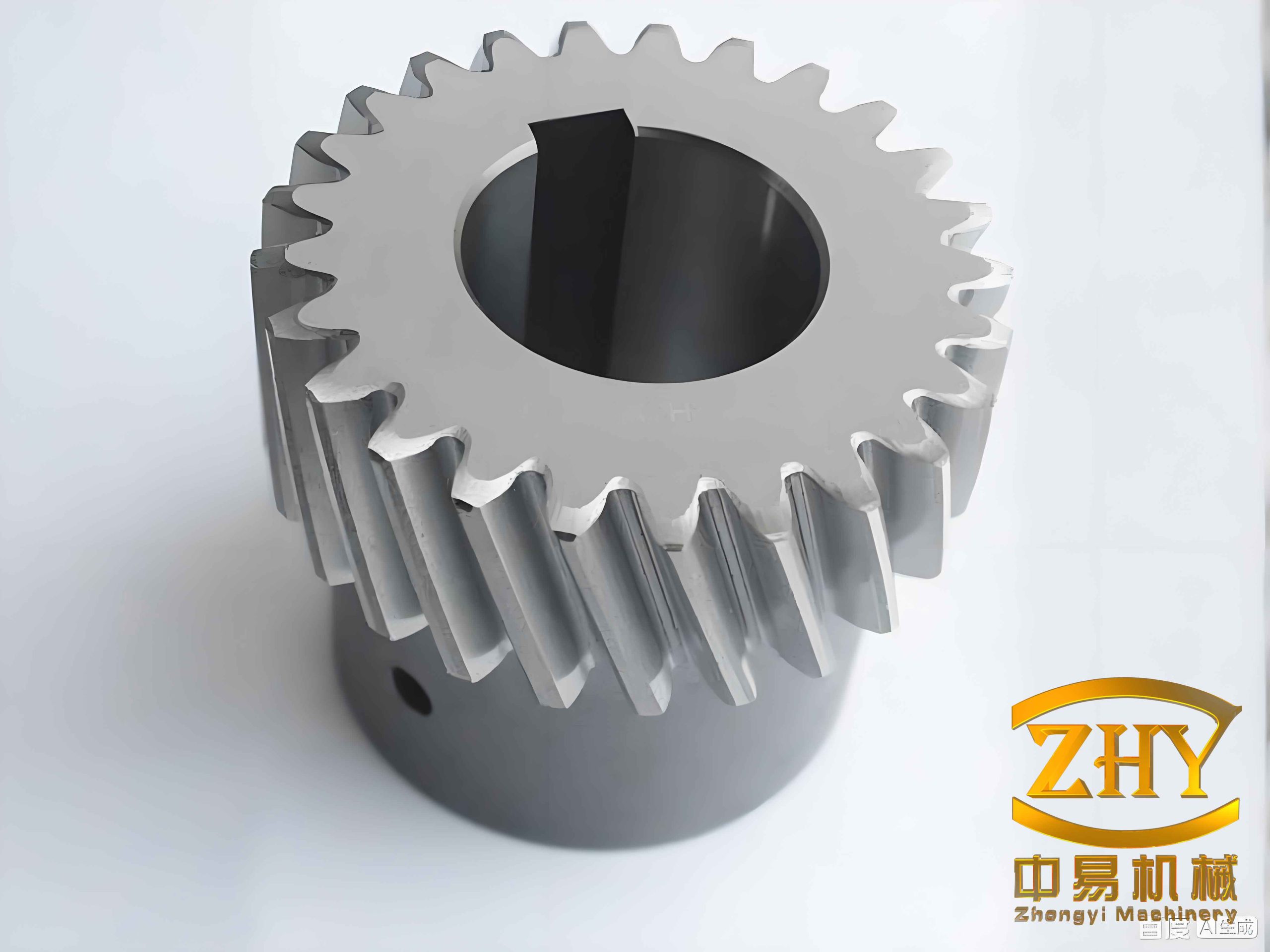
The figure above shows a representative helical gear. In my analysis, the helical gear is not treated as a simple spur gear with an inclined tooth. Instead, I explicitly account for the helix angle, the axial mesh force component, the contact line variation along the tooth width, and the load-dependent nonlinear Hertzian contact behavior. These factors are essential for obtaining an accurate time-varying meshing stiffness of a helical gear pair.
1. Improved Time-Varying Meshing Stiffness of a Healthy Helical Gear
I begin with the slicing model. A helical gear is divided along the tooth width into a finite number of thin slices. Each slice is sufficiently thin that its helix angle can be neglected, and therefore each slice can be treated as a spur gear slice. If the total face width is \(W\) and the number of slices is \(m\), then the thickness of each slice is
$$ \Delta w = \frac{W}{m}. $$
For each slice, I calculate the local mesh stiffness by using the potential energy method. The total mesh stiffness of the helical gear pair is then obtained by summing the contributions of all slices that are simultaneously in contact. Because the contact line of a helical gear changes length during the meshing cycle, the number of active slices also changes with the rotation angle. This is one of the main differences between a helical gear and a spur gear.
1.1 Tooth Profile Equations
To calculate the tooth stiffness accurately, I need the exact tooth profile of a single slice. The tooth profile consists of a transition curve near the root and an involute curve on the working flank. For the transition curve, I use the following parametric equations:
$$
\begin{aligned}
x &= r \left[ \cos(\phi) + \left( \frac{A}{r} \right) \sin(\phi) – \frac{A}{r} \right], \\
y &= r \left[ \sin(\phi) – \left( \frac{A}{r} \right) \cos(\phi) \right],
\end{aligned}
$$
where \(r\) is the pitch radius, \(\phi\) is the parameter, and \(A\) is determined by the cutter geometry and the tooth addendum. For the involute portion, the coordinates of any point \(K\) can be written as
$$
\begin{aligned}
x_K &= r_K \cos\left( \frac{\pi}{2} – \theta_K – N_K \right), \\
y_K &= r_K \sin\left( \frac{\pi}{2} – \theta_K – N_K \right),
\end{aligned}
$$
where \(r_K = r_b / \cos(\alpha_K)\), \(r_b\) is the base radius, \(\alpha_K\) is the pressure angle at point \(K\), and \(\theta_K = \tan(\alpha_K) – \alpha_K\). The parameter \(N_K\) is defined by
$$ N_K = \beta + \frac{\pi}{2} – \theta_K – \theta, $$
where \(\beta\) describes the angular position of the tooth center line relative to the tangent line of the base circle. By using these equations, I generate the complete single-tooth profile for each slice of the helical gear. This profile is then used to calculate the bending, shear, and axial compression stiffnesses.
1.2 Time-Varying Contact Line of a Helical Gear
The contact line of a helical gear pair is inclined with respect to the gear axis. For a single tooth pair, the contact line length changes from zero to a maximum value and then decreases to zero. The total contact ratio of a helical gear is
$$ \varepsilon_\gamma = \varepsilon_\alpha + \varepsilon_\beta, $$
where \(\varepsilon_\alpha\) is the transverse contact ratio and \(\varepsilon_\beta\) is the overlap contact ratio. The overlap contact ratio is given by
$$ \varepsilon_\beta = \frac{W \sin(\beta)}{m_n \pi}, $$
where \(\beta\) is the helix angle and \(m_n\) is the normal module. The transverse contact ratio is
$$ \varepsilon_\alpha = \frac{1}{2\pi} \left[ N_1 \left( \tan(\alpha_{at1}) – \tan(\alpha_t) \right) + N_2 \left( \tan(\alpha_{at2}) – \tan(\alpha_t) \right) \right], $$
where \(N_1\) and \(N_2\) are the numbers of teeth of the pinion and gear, \(\alpha_{at1}\) and \(\alpha_{at2}\) are the transverse addendum pressure angles, and \(\alpha_t\) is the transverse pressure angle. For a single tooth pair, the meshing period is
$$ \theta_p = \frac{2\pi \varepsilon_\gamma}{N_1}. $$
When \(\varepsilon_\beta \le \varepsilon_\alpha\), the contact line length of a single tooth pair can be expressed in three intervals as
$$
L(t)=
\begin{cases}
\frac{W}{\sin(\beta_b)}, & t_1 \le t \le t_2, \\[4pt]
\frac{W}{\cos(\beta_b)}, & t_2 \le t \le t_5, \\[4pt]
\frac{(N_1 t + 2\pi \varepsilon_\alpha)}{\sin(\beta_b)}, & t_5 \le t \le t_6,
\end{cases}
$$
where \(\beta_b\) is the base helix angle. When \(\varepsilon_\beta \ge \varepsilon_\alpha\), the contact line length becomes
$$
L(t)=
\begin{cases}
\frac{W}{\sin(\beta_b)}, & t_1 \le t \le t_2, \\[4pt]
\frac{N_1 t + 2\pi \varepsilon_\alpha}{\sin(\beta_b)}, & t_2 \le t \le t_5, \\[4pt]
\frac{(N_1 t + 2\pi \varepsilon_\gamma)}{\sin(\beta_b)}, & t_5 \le t \le t_6.
\end{cases}
$$
The total contact line length at time \(t\) is the sum of the contact line lengths of all tooth pairs that are simultaneously in mesh:
$$ L_{\text{total}}(t) = \sum_{i=1}^{5} L_i(t). $$
This total contact line length controls the number of active slices and therefore has a direct influence on the time-varying meshing stiffness of the helical gear pair.
1.3 Stiffness Components from Potential Energy
For a single slice, I decompose the tooth stiffness into bending stiffness \(k_b\), shear stiffness \(k_s\), axial compression stiffness \(k_a\), foundation stiffness \(k_f\), and Hertzian contact stiffness \(k_h\). The bending, shear, and axial compression stiffnesses are obtained from the potential energy method:
$$
\begin{aligned}
U_b &= \frac{1}{k_b} = \int \frac{M^2}{2EI} \, dx, \\
U_s &= \frac{1}{k_s} = \int \frac{1.2 F^2}{2GA} \, dx, \\
U_a &= \frac{1}{k_a} = \int \frac{F_a^2}{2EA} \, dx.
\end{aligned}
$$
For the transition curve and the involute curve, the cross-sectional area and moment of inertia are
$$
\begin{aligned}
A_1 &= 2 y_1 \Delta w, & I_1 &= \frac{2}{3} y_1^3 \Delta w, \\
A_2 &= 2 y_2 \Delta w, & I_2 &= \frac{2}{3} y_2^3 \Delta w.
\end{aligned}
$$
After substituting the torque and force components, the bending stiffness of a single slice can be written as
$$
\frac{1}{k_b} = \int_{x_A}^{x_B} \frac{\left( x_{Pm} – x \right)^2 \cos^2(\alpha_{Pm})}{EI_x} \, dx,
$$
and the shear stiffness is
$$
\frac{1}{k_s} = \int_{x_A}^{x_B} \frac{1.2 \cos^2(\alpha_{Pm})}{G A_x} \, dx.
$$
The axial compression stiffness is
$$
\frac{1}{k_a} = \int_{x_A}^{x_B} \frac{\sin^2(\alpha_{Pm})}{E A_x} \, dx.
$$
These three stiffnesses are connected in series to form the tooth stiffness of a single slice:
$$ \frac{1}{k_t} = \frac{1}{k_a} + \frac{1}{k_b} + \frac{1}{k_s}. $$
1.4 Load-Dependent Hertzian Contact Stiffness
In many simplified models, the Hertzian contact stiffness is treated as a constant. I improve this by using a load-dependent nonlinear Hertzian contact stiffness:
$$ k_h = \frac{E^{0.9} \Delta w^{0.8} F_i^{0.1}}{1.275}. $$
Here \(F_i\) is the load carried by the \(i\)-th slice,
$$ F_i = F_t’ \, lsr_i, $$
where \(lsr_i\) is the load sharing ratio. This expression shows that the Hertzian contact stiffness of a helical gear depends not only on the material and tooth width but also on the instantaneous contact force. Therefore, the helical gear mesh stiffness is intrinsically nonlinear and time-varying.
1.5 Foundation Stiffness and Multi-Tooth Correction
The foundation stiffness of a single tooth pair is calculated by the analytical formula
$$
\frac{1}{k_f} = \frac{\cos^2(\alpha_{Pm})}{E W} \left[ L^* \left( \frac{u_f}{S_f} \right)^2 + M^* \left( \frac{u_f}{S_f} \right) + P^* \left( \frac{u_f}{S_f} \right) + Q^* \tan^2(\alpha_{Pm}) \right].
$$
This formula is accurate for a single tooth pair, but it overestimates the foundation stiffness when multiple tooth pairs mesh simultaneously. I therefore introduce a correction coefficient \(C_f^*\):
$$ k_f’ = \frac{1}{C_f^*} k_f. $$
The corrected foundation stiffness \(k_f’\) is used for each tooth pair in the multi-tooth mesh region. The single-slice stiffness of a healthy helical gear is then
$$
k = \frac{1}{\frac{1}{k_{tp}} + \frac{1}{k_{fp}’} + \frac{1}{k_h} + \frac{1}{k_{tg}} + \frac{1}{k_{fg}’}}.
$$
For a single tooth pair of the helical gear, the stiffness is obtained by summing all active slices:
$$ K’ = \sum_{i=i_1}^{i_2} k_i. $$
Finally, because the axial force component affects the deformation of the helical gear, I apply a correction based on the base helix angle:
$$ K = K’ \cos^2(\beta_b). $$
The total time-varying meshing stiffness of the helical gear pair is then
$$ K_{\text{total}}(t) = \sum_{i=1}^{5} K_i(t). $$
1.6 Parametric Study of Healthy Helical Gear Stiffness
I study how the geometric parameters of a helical gear influence the single-tooth stiffness and the total mesh stiffness. The reference parameters are listed in Table 1.
| Parameter | Pinion | Gear |
|---|---|---|
| Number of teeth \(N\) | 34 | 52 |
| Normal module \(m_n\) (mm) | 2 | 2 |
| Face width \(W\) (mm) | 12 | 12 |
| Normal pressure angle \(\alpha_n\) (deg) | 20 | 20 |
| Helix angle \(\beta\) (deg) | 15 | 15 |
| Addendum coefficient \(h_{an}^*\) | 1 | 1 |
| Clearance coefficient \(c_n^*\) | 0.25 | 0.25 |
| Young’s modulus \(E\) (Pa) | \(2.0\times 10^{11}\) | \(2.0\times 10^{11}\) |
| Poisson’s ratio \(\nu\) | 0.3 | 0.3 |
| Inner radius \(r_i\) (mm) | 15 | 15 |
| Torque \(T\) (N m) | 100 | 100 |
| Total contact ratio \(\varepsilon_\gamma\) | 2.1321 | 2.1321 |
Table 2 summarizes the qualitative trends that I observe when changing the module, helix angle, face width, pressure angle, and inner hole radius. These trends are important for the design of helical gear pairs because they show how the mesh stiffness can be tuned by geometry.
| Parameter change | Effect on single-tooth stiffness | Effect on total mesh stiffness | Main reason |
|---|---|---|---|
| Increase module | Decreases | Decreases | Larger radii reduce normal and axial forces for a given torque |
| Increase helix angle | Decreases slightly | Nearly unchanged | Normal and axial forces increase, but total contact ratio also increases |
| Increase face width | Increases | Increases significantly | Load per unit width decreases and contact ratio increases |
| Increase pressure angle | Increases | Increases | Tooth bending, shear, and axial stiffnesses change favorably |
| Increase inner hole radius | Increases | Increases | Foundation flexibility decreases |
For example, when the module changes from 2 mm to 6 mm, the total contact ratio decreases from about 2.13 to 1.80, and the single-tooth mesh stiffness decreases. When the face width increases from 10 mm to 30 mm, the total contact ratio increases from about 2.05 to 2.87, and both the single-tooth and total mesh stiffnesses increase significantly. When the pressure angle increases from 15 degrees to 25 degrees, the total contact ratio decreases from about 2.43 to 1.94, but the mesh stiffness increases because the tooth stiffness components become larger.
I also examine the influence of the inner hole radius. The analytical foundation stiffness formula is valid for
$$ 1.4 \le \frac{r_f}{r_{\text{int}}} \le 7. $$
For the reference helical gear, the root radius is about 32.70 mm. I choose inner hole radii of 10 mm, 13 mm, and 16 mm. As the inner hole radius increases, the foundation deformation decreases, the foundation stiffness increases, and the mesh stiffness of the helical gear increases. This result is consistent with the physical expectation that a stiffer gear body supports the tooth more effectively.
1.7 Finite Element Validation for Healthy Helical Gear
I validate my theoretical method by using a commercial finite element code. A three-dimensional model of the helical gear pair is generated, and the material properties are assigned according to Table 1. The contact surfaces are defined as frictional contacts with a friction coefficient of 0.2. The mesh is refined near the contact zones. The driven gear is fully fixed, while the driving gear is allowed to rotate only about its central axis. A torque of 100 N m is applied to the driving gear. The finite element mesh stiffness is calculated from
$$ k_{\text{finite}} = \frac{T}{r_b \theta_p}, $$
where \(\theta_p\) is the rotation angle of the driving gear obtained from the finite element analysis. The comparison between my analytical method and the finite element method shows good agreement. The maximum error is about 1.71 percent. This validates the proposed time-varying meshing stiffness model for a healthy helical gear.
2. Time-Varying Meshing Stiffness of a Helical Gear with Pitting and Spalling
Pitting and spalling are common surface faults in helical gears. When a helical gear tooth surface is pitted, the effective contact line is shortened, the Hertzian contact stiffness is reduced, and the cross-sectional area and area moment of inertia of the tooth are decreased. As a result, the time-varying meshing stiffness of the helical gear decreases in the pitted region. To capture this effect accurately, I propose three pitting models: a special ellipsoid model, a general ellipsoid model, and an irregular pitting model.
2.1 Special Ellipsoid Pitting Model
In the special ellipsoid model, the ellipsoid intersects the tooth surface to form an ellipse whose major axis is parallel to the contact line. The maximum pitting width, maximum pitting length, and maximum pitting depth are denoted by \(w_{s,\max}\), \(l_{s,\max}\), and \(h_{s,\max}\), respectively. The ellipsoid radii in the local coordinate system are
$$
\begin{aligned}
a &= b = r_s = \frac{1}{2} \sqrt{h_{s,\max}^2 + w_{s,\max}^2}, \\
c &= \frac{1}{2} \sqrt{l_{s,\max}^2 + h_{s,\max}^2}.
\end{aligned}
$$
For a given meshing position \(x_s\), the pitting depth is
$$ h_{xsk} = \sqrt{r_{s,\max}^2 – \left( (x_s – x_1)\cos(\beta_b) \right)^2} – \left( r_{s,\max} – h_{s,\max} \right). $$
The reduced area of the pitting cross-section is
$$ A_{xsk} = \int_{-b_{xsk}}^{b_{xsk}} 2 c_{xsk} \sqrt{1 – \frac{y’^2}{b_{xsk}^2}} \, dy’, $$
where \(b_{xsk}\) and \(c_{xsk}\) are the semi-axes of the elliptical pitting section. By using the equivalent area method, the equivalent reduction in tooth height is
$$ h_s = \frac{A_{xsk}}{l_s}, $$
where \(l_s\) is the pitting length at position \(x_s\). The pitted slice stiffness is then calculated by replacing the original cross-sectional area and moment of inertia with
$$
\begin{aligned}
A_{xs} &= (2 y_{xs} – h_s) \Delta w, \\
I_{xs} &= \frac{1}{12} \Delta w (2 y_{xs} – h_s)^3.
\end{aligned}
$$
The corresponding bending, shear, and axial compression stiffnesses are obtained by substituting these reduced section properties into the potential energy integrals.
2.2 General Ellipsoid Pitting Model
In the general ellipsoid model, the ellipse formed on the tooth surface is not parallel to the contact line. There is an angle \(\alpha\) between the major axis of the ellipse and the contact line. The ellipse equation in the \(x-z\) plane is
$$
\frac{\left( (x-x_0)\cos\alpha + (z-z_0)\sin\alpha \right)^2}{a^2}
+
\frac{\left( -(x-x_0)\sin\alpha + (z-z_0)\cos\alpha \right)^2}{c^2}
= 1.
$$
The intersection between the contact line and the ellipse gives the start and end points of the pitting region. The pitting length at position \(x_s\) is
$$ l_s = \sqrt{(x_1 – x_2)^2 + (z_1 – z_2)^2}. $$
The maximum pitting depth at that position is
$$ h_{xsk} = 2 b_s \sqrt{1 – \frac{l_s^2}{4 c_s^2}}. $$
By using the same equivalent area method, I obtain the reduced height and the modified section properties. The general ellipsoid model is more flexible than the special ellipsoid model because it can represent pitting at arbitrary orientations on the helical gear tooth surface.
2.3 Irregular Pitting Model
Real pitting shapes are often irregular. To represent them, I divide the pitting boundary into two curves \(a(x)\) and \(b(x)\). By measuring discrete pitting lengths along the tooth surface and fitting polynomials, I obtain
$$
\begin{aligned}
a(x) &= p_n x^n + p_{n-1} x^{n-1} + \cdots + p_1 x + p_0, \\
b(x) &= q_n x^n + q_{n-1} x^{n-1} + \cdots + q_1 x + q_0.
\end{aligned}
$$
The intersection of the contact line with these two curves gives the pitting boundaries at each meshing position. The pitting depth can be treated as a constant or as a function of position. The irregular model is the most general of the three models and can be applied to measured pitting shapes from real helical gear failures.
2.4 Stiffness Reduction due to Pitting
For a pitted slice, the tooth stiffness is calculated as
$$ \frac{1}{k_{ts}} = \frac{1}{k_{as}} + \frac{1}{k_{bs}} + \frac{1}{k_{ss}}, $$
where \(k_{as}\), \(k_{bs}\), and \(k_{ss}\) are the axial compression, bending, and shear stiffnesses of the pitted slice. The total stiffness of one tooth pair in the pitted region is
$$ k_{\text{total}} = \frac{1}{\frac{1}{k_{tsp}} + \frac{1}{k_{fp}} + \frac{1}{k_{tg}} + \frac{1}{k_{fg}}}. $$
The single-tooth pair stiffness in the pitted region is then summed over all active slices, and the total helical gear mesh stiffness is obtained by summing all simultaneously meshing tooth pairs. The pitting reduces the mesh stiffness mainly because the Hertzian contact is removed in the pitted area, and because the tooth cross-section is smaller. The foundation stiffness is not directly affected by pitting because the gear body remains intact.
2.5 Finite Element Validation for Pitted Helical Gears
I validate the pitting models by using finite element analysis. Four cases are considered: special ellipsoid model 1, special ellipsoid model 2, general ellipsoid model, and irregular model. Table 3 lists the pitting parameters and the maximum error between my analytical method and the finite element method.
| Pitting model | Center or key position | Maximum pitting width (mm) | Maximum pitting length (mm) | Orientation angle (deg) | Maximum error (%) |
|---|---|---|---|---|---|
| Special ellipsoid 1 | (5, 6) | 3.74 | 4 | 0 | 3.01 |
| Special ellipsoid 2 | (5, 6) | 3.74 | 8 | 0 | 3.97 |
| General ellipsoid | (5, 6) | 3.74 | 4 | 10 | 4.48 |
| Irregular | left end (4.1, 5.5) | variable | variable | irregular | 2.80 |
The results show that pitting significantly reduces the time-varying meshing stiffness of the helical gear in the pitted meshing region. For the special ellipsoid model, the minimum mesh stiffness is about \(1.504\times 10^8\) N/m for a pitting length of 4 mm and about \(1.299\times 10^8\) N/m for a pitting length of 8 mm. The difference is about 15.8 percent, which demonstrates that the pitting length strongly affects the severity of the stiffness loss. The general ellipsoid model produces a wider pitted meshing region because the ellipse is inclined relative to the contact line. The irregular model produces its own characteristic stiffness reduction, and the analytical result agrees with the finite element result within 2.8 percent.
3. Compound Transmission Stiffness of a Gear-Shaft System
In a real transmission system, the helical gear pair is not isolated. It is connected to input and output shafts. The shaft stiffness and the gear mesh stiffness interact, and the compound transmission stiffness cannot be obtained by simply connecting the pinion shaft, the gear mesh, and the gear shaft in series. I therefore develop a compound transmission stiffness model for a gear-shaft system.
The gear mesh stiffness calculated by the potential energy method is a rectilinear stiffness. It is converted into a torsional stiffness by
$$ k_{\text{torsional}} = r_b^2 k_{\text{rectilinear}}. $$
For a gear-shaft system, the total twist angle is
$$ \theta_{\text{total}} = \theta_1 + \theta_{pg} + \theta_2 i, $$
where \(\theta_1\) is the twist angle of the driving shaft, \(\theta_{pg}\) is the twist angle of the gear pair, \(\theta_2\) is the twist angle of the driven shaft, and \(i\) is the transmission ratio. The individual twist angles are
$$
\theta_1 = \frac{T_1}{k_1}, \quad
\theta_{pg} = \frac{T_1}{k_n}, \quad
\theta_2 = \frac{T_1 i}{k_2}.
$$
Therefore, the compound transmission stiffness of the gear-shaft system is
$$ \frac{1}{k_{\text{total}}} = \frac{1}{k_1} + \frac{1}{k_n} + \frac{i^2}{k_2}. $$
For a solid gear pair, the mesh stiffness itself can be decomposed into the driving shaft segment, the gear mesh, and the driven shaft segment:
$$ k_n = k_{\text{shaft},p} + k_{pg} + k_{\text{shaft},g}. $$
This compound model is important because the driving and driven shafts often have different diameters and lengths, and the numbers of teeth on the pinion and gear are different. The transmission ratio therefore appears explicitly in the compound stiffness expression.
3.1 Experimental Platform for Compound Transmission Stiffness
I design and manufacture an experimental platform to validate the compound transmission stiffness method. The platform consists of a support platform, a loading unit, a single-stage cylindrical gear reducer, an end-fixing unit, and a rotation-angle measurement unit. The loading unit applies a known torque to the driving shaft through a lever and a force sensor. The end-fixing unit holds the driven shaft fixed. Four laser position sensors are installed on the driving and driven shafts to measure the twist angles before and after loading.
The applied torque is
$$ T = F L, $$
where \(F\) is the force measured by the sensor and \(L\) is the lever length. The rotation angle is obtained from the laser spot displacement on a distant wall:
$$ \theta = \arctan\left( \frac{\Delta L}{L} \right), $$
where \(\Delta L\) is the displacement of the laser spot and \(L\) is the distance from the shaft center to the wall. Because the angle is small, this can be approximated as
$$ \theta \approx \frac{\Delta L}{L}. $$
The total compound twist angle of the gear-shaft system is
$$ \theta_{\text{total,exp}} = (\theta_{s1} – \theta_{s2}) + i(\theta_{s3} – \theta_{s4}). $$
The experimental compound transmission stiffness is then
$$ k_{\text{total,exp}} = \frac{T}{\theta_{\text{total,exp}}}. $$
I use two gear-shaft pairs with different modules and numbers of teeth. The shaft parameters are listed in Table 4, and the gear parameters are listed in Table 5.
| Parameter | Driving shaft | Driven shaft |
|---|---|---|
| Length \(L_1\), \(L_2\) (mm) | 70 | 85 |
| Diameter \(D_1\), \(D_2\) (mm) | 50 | 60 |
| Parameter | Gear pair 1 pinion | Gear pair 1 gear | Gear pair 2 pinion | Gear pair 2 gear |
|---|---|---|---|---|
| Number of teeth \(N\) | 40 | 60 | 20 | 30 |
| Normal module \(m_n\) (mm) | 2.5 | 2.5 | 5 | 5 |
| Face width \(W\) (mm) | 45 | 45 | 45 | 45 |
The experimental and theoretical results show good agreement. The twist angle and the compound transmission stiffness follow the same trend. The experimental results exhibit some scatter because of manual loading, support bearing flexibility, and small shear and bending deformations of the shafts. Nevertheless, the comparison validates both the theoretical compound transmission stiffness model and the experimental platform.
4. Thirteen-Degree-of-Freedom Dynamic Model of a Helical Gear System
I build a refined thirteen-degree-of-freedom dynamic model of a helical gear transmission system. The model includes the driving motor, coupling, shafts, bearings, helical gear pair, load, and gearbox housing. The generalized displacement vector is
$$ \mathbf{q} = \{ \theta_M, \theta_p, \theta_g, \theta_L, x_p, y_p, z_p, x_g, y_g, z_g, x_f, y_f, z_f \}. $$
The model includes four rotational degrees of freedom and nine translational degrees of freedom. The gearbox housing is connected to the support through four bolts. Each bolt has stiffness and damping in the \(x\), \(y\), and \(z\) directions. The helical gear pair is connected by a mesh spring and a mesh damper, and the dynamic mesh force is
$$ F_{pg} = k_m \delta_m + c_m \dot{\delta}_m, $$
where \(k_m\) is the total mesh stiffness of the helical gear and \(c_m\) is the mesh damping. The dynamic transmission error is
$$ \delta_m = \frac{\delta_t}{\cos \beta_b}, $$
with
$$ \delta_t = R_{bp}\theta_p – R_{bg}\theta_g + (x_p – x_g)\cos\varphi + (y_p – y_g)\sin\varphi – e(t). $$
The mesh damping is calculated from
$$ c_m = 2 \xi_g \sqrt{\frac{k_m R_{bp}^2 R_{bg}^2 I_p I_g}{R_{bp}^2 I_p + R_{bg}^2 I_g}}. $$
The equations of motion for the rotational degrees of freedom are
$$
\begin{aligned}
I_M \ddot{\theta}_M + c_{pb}(\dot{\theta}_M – \dot{\theta}_p) + k_{pb}(\theta_M – \theta_p) &= T_M, \\
I_p \ddot{\theta}_p + c_{pb}(\dot{\theta}_p – \dot{\theta}_M) + k_{pb}(\theta_p – \theta_M) &= -R_{bp}F_{pg} – M_p, \\
I_g \ddot{\theta}_g + c_{gb}(\dot{\theta}_g – \dot{\theta}_L) + k_{gb}(\theta_g – \theta_L) &= R_{bg}F_{pg} + M_g, \\
I_L \ddot{\theta}_L + c_{gb}(\dot{\theta}_L – \dot{\theta}_g) + k_{gb}(\theta_L – \theta_g) &= -T_L.
\end{aligned}
$$
The translational equations for the pinion, gear, and gearbox are written in a similar manner. The mesh force components along the coordinate axes are
$$
\begin{aligned}
F_{mx} &= F_{pg} \cos\beta_b \cos\alpha, \\
F_{my} &= F_{pg} \cos\beta_b \sin\alpha, \\
F_{mz} &= F_{pg} \sin\beta_b.
\end{aligned}
$$
The bearing forces and gearbox bolt forces are included as spring-damper connections. The gearbox housing has three translational degrees of freedom, and its vibration is coupled to the gear pair through the bearings and bolts.
4.1 Friction Excitation under Elastohydrodynamic Lubrication
I include friction excitation because the helical gear pair operates under elastohydrodynamic lubrication. The friction coefficient is calculated by a mixed elastohydrodynamic lubrication model. For each slice, the friction force is
$$ F_{fpi} = F_{fgi} = \mu_i F_{pgi}, $$
where \(\mu_i\) is the instantaneous friction coefficient. The friction coefficient is expressed as
$$ \mu_i = e^{b_1} S^{b_2} P_h^{b_3} V_e^{b_4} v_r^{b_5} R^{b_6} \left( \frac{S}{S_0} \right)^{b_7} \left( \frac{P_h}{P_{h0}} \right)^{b_8} \left( \frac{V_e}{V_{e0}} \right)^{b_9}. $$
The regression coefficients are
$$ [b_1, b_2, \ldots, b_9] = [-8.92, 1.03, 1.04, -0.35, 2.81, -0.1, 0.75, -0.39, 0.62]. $$
The surface roughness of a pitted helical gear is modified as
$$ S_{g,\text{spall}} = S_{\text{healthy}} \frac{L}{L_{\text{spall}}}. $$
This means that when pitting occurs, the local surface roughness increases, the friction coefficient increases, and the friction force and friction moment become larger. The friction moment on the pinion and gear is
$$
\begin{aligned}
M_p &= \sum_{i=1}^{n} r_{pm} F_{fpi}, \\
M_g &= \sum_{i=1}^{n} r_{gm} F_{fgi}.
\end{aligned}
$$
The total friction force is
$$ F_f = \sum_{i=1}^{n} F_{fpi}. $$
These friction excitations are added to the dynamic equations. They affect the rotational and translational vibrations of the helical gear system, especially in the pitted region.
4.2 Healthy Vibration Response
I solve the thirteen-degree-of-freedom dynamic equations by using a stiff ordinary differential equation solver. The dynamic mesh force, displacement, velocity, and acceleration responses are obtained for the healthy helical gear system. The input speed is 6000 rpm. The theoretical meshing frequency is
$$ f_m = \frac{n N_1}{60} = \frac{6000 \times 34}{60} = 3400\ \text{Hz}. $$
The input shaft frequency is
$$ f_s = \frac{n}{60} = 100\ \text{Hz}, $$
and the output shaft frequency is
$$ f_{s1} = \frac{f_s}{i} = 65.4\ \text{Hz}. $$
The dynamic mesh force fluctuates around 56500 N, while the theoretical average mesh force is about 54647 N. This agreement confirms that the dynamic model is reliable. The frequency spectrum of the dynamic mesh force shows a dominant peak at about 340.1 Hz, which is very close to the theoretical meshing frequency of 340 Hz.
The displacement, velocity, and acceleration responses of the pinion, gear, and gearbox are also obtained. The pinion and gear have larger translational vibration amplitudes than the gearbox because the gearbox is bolted to the support. The gearbox translational vibrations oscillate around zero, while the pinion and gear vibrations are shifted because of the mean mesh force. The angular acceleration of the pinion is larger than that of the gear because the pinion rotates at a higher speed.
4.3 Pitting Vibration Response
I analyze four pitting cases: general ellipsoid pitting 1, general ellipsoid pitting 2, special ellipsoid pitting, and irregular pitting. In all cases, the dynamic mesh force exhibits periodic fluctuations in the pitted region. As the pitting length increases, the fluctuation amplitude increases. The friction force and friction moment also increase in the pitted region because the surface roughness increases and the effective contact line decreases.
The gearbox acceleration response is especially important because in real measurements the sensors are usually mounted on the gearbox surface. I therefore analyze the gearbox acceleration in the \(x\), \(y\), and \(z\) directions. The time-domain results show periodic impulses in all three directions. The impulse timing coincides with the pitting engagement, and the impulse amplitude increases with the severity of the pitting.
In the frequency domain, I apply the fast Fourier transform to the gearbox acceleration. The spectra show sidebands around the meshing frequency. This is a typical signature of localized tooth faults in a helical gear. The sidebands are caused by the periodic impact produced when the pitted tooth enters the mesh. The presence of these sidebands confirms that the proposed dynamic model can capture the vibration characteristics of a pitted helical gear system.
4.4 Key Results and Discussion
Table 6 summarizes the main dynamic response features under healthy and pitted conditions.
| Condition | Dynamic mesh force | Friction force | Friction moment | Gearbox acceleration | Frequency-domain feature |
|---|---|---|---|---|---|
| Healthy helical gear | Almost periodic, small fluctuation | Small and smooth | Small and smooth | Low-level periodic vibration | Dominant mesh frequency |
| Special ellipsoid pitting | Periodic drop in pitted region | Local increase | Local increase | Periodic impulse | Sidebands around mesh frequency |
| General ellipsoid pitting | Larger fluctuation | Higher local increase | Higher local increase | Stronger impulse | Wider sidebands |
| Irregular pitting | Irregular fluctuation | Irregular increase | Irregular increase | Irregular impulse | Multiple modulation features |
I find that the pitting length is one of the most important parameters affecting the dynamic response. As the pitting length increases, the effective contact line becomes shorter, the helical gear mesh stiffness decreases further, and the dynamic mesh force fluctuation becomes larger. At the same time, the elastohydrodynamic lubrication condition changes because the surface roughness increases in the pitted region. This leads to larger friction forces and friction moments. The gearbox acceleration response is therefore more impulsive, and the sidebands around the meshing frequency become more pronounced.
Another important finding is that the foundation stiffness of the helical gear is not directly affected by pitting because the gear body remains intact. The main stiffness reduction comes from the loss of Hertzian contact in the pitted area and the reduction of the tooth cross-sectional area and area moment of inertia. This means that the pitting model must accurately represent the pitted area and the equivalent reduction in tooth height. My equivalent area method provides a practical way to do this.
The compound transmission stiffness of the gear-shaft system also plays a role in the dynamic response. Because the pinion and gear shafts have different lengths and diameters, and because the pinion and gear have different numbers of teeth, the compound stiffness is not a simple series combination. The transmission ratio appears explicitly in the compound stiffness formula, and the shaft stiffness affects the overall torsional vibration of the helical gear system. The experimental platform confirms that the compound transmission stiffness model is reliable.
5. Conclusions
I have developed a complete framework for the mesh stiffness calculation and dynamic analysis of healthy and pitted helical gears. The main conclusions are as follows.
First, I proposed an improved time-varying meshing stiffness method for a healthy helical gear. The method is based on the slicing model and the potential energy method. It includes a load-dependent Hertzian contact stiffness, a correction for repeated foundation stiffness in multi-tooth meshing, and a correction for the axial force component. The method was validated by finite element analysis, with a maximum error of about 1.71 percent. The parametric study showed that the module, helix angle, face width, pressure angle, and inner hole radius all influence the helical gear mesh stiffness.
Second, I proposed three pitting models for helical gears: a special ellipsoid model, a general ellipsoid model, and an irregular model. These models are more realistic than simple rectangular or circular pitting models because they allow curved pitting bottoms, arbitrary orientation, and irregular boundaries. The equivalent area method was used to calculate the reduced cross-sectional area and area moment of inertia. The finite element validation showed that the proposed models can accurately calculate the time-varying meshing stiffness of a pitted helical gear. The pitting length was found to be a key factor controlling the severity of the stiffness reduction.
Third, I explored the compound transmission stiffness of a gear-shaft system. I showed that the gear mesh stiffness must be converted into a torsional stiffness, and that the shaft stiffnesses and the gear mesh stiffness must be combined through the transmission ratio. The compound stiffness formula is
$$ \frac{1}{k_{\text{total}}} = \frac{1}{k_1} + \frac{1}{k_n} + \frac{i^2}{k_2}. $$
I designed and manufactured an experimental platform to validate this formula. The experimental results and theoretical results agreed well, confirming the accuracy of the compound transmission stiffness model.
Fourth, I built a thirteen-degree-of-freedom dynamic model of a helical gear transmission system. The model includes elastohydrodynamic lubrication friction excitation and gearbox coupling effects. The dynamic mesh force, displacement, velocity, and acceleration responses were obtained for healthy and pitted conditions. The frequency spectra of the gearbox acceleration showed sidebands around the meshing frequency when pitting occurred. The pitting length, pitting shape, and surface roughness all influenced the friction force, friction moment, and gearbox vibration. The proposed model provides a useful tool for understanding the vibration mechanism of pitted helical gears and for developing fault diagnosis methods.
Overall, my research shows that accurate modeling of the time-varying meshing stiffness of a helical gear is essential for predicting the dynamic behavior of a geared transmission system. The pitting shape, the load-dependent contact stiffness, the multi-tooth foundation correction, the axial force correction, the compound gear-shaft stiffness, and the elastohydrodynamic friction excitation all must be considered together. The methods and results presented here can be used for the design, condition monitoring, and fault severity assessment of helical gear systems.