
The precise control of transmission error stands as a pivotal technical challenge in the design and manufacture of high-precision rotary vector (RV) reducers. In this study, we employ a comprehensive methodology combining virtual prototyping and orthogonal experimental design to investigate the influence of key component manufacturing and assembly errors on the overall transmission accuracy of an RV reducer. Our objective is to determine the hierarchy of influence among various error factors, derive a reliable calculation formula for transmission error, and thereby provide a theoretical foundation for guiding manufacturing tolerance allocation.
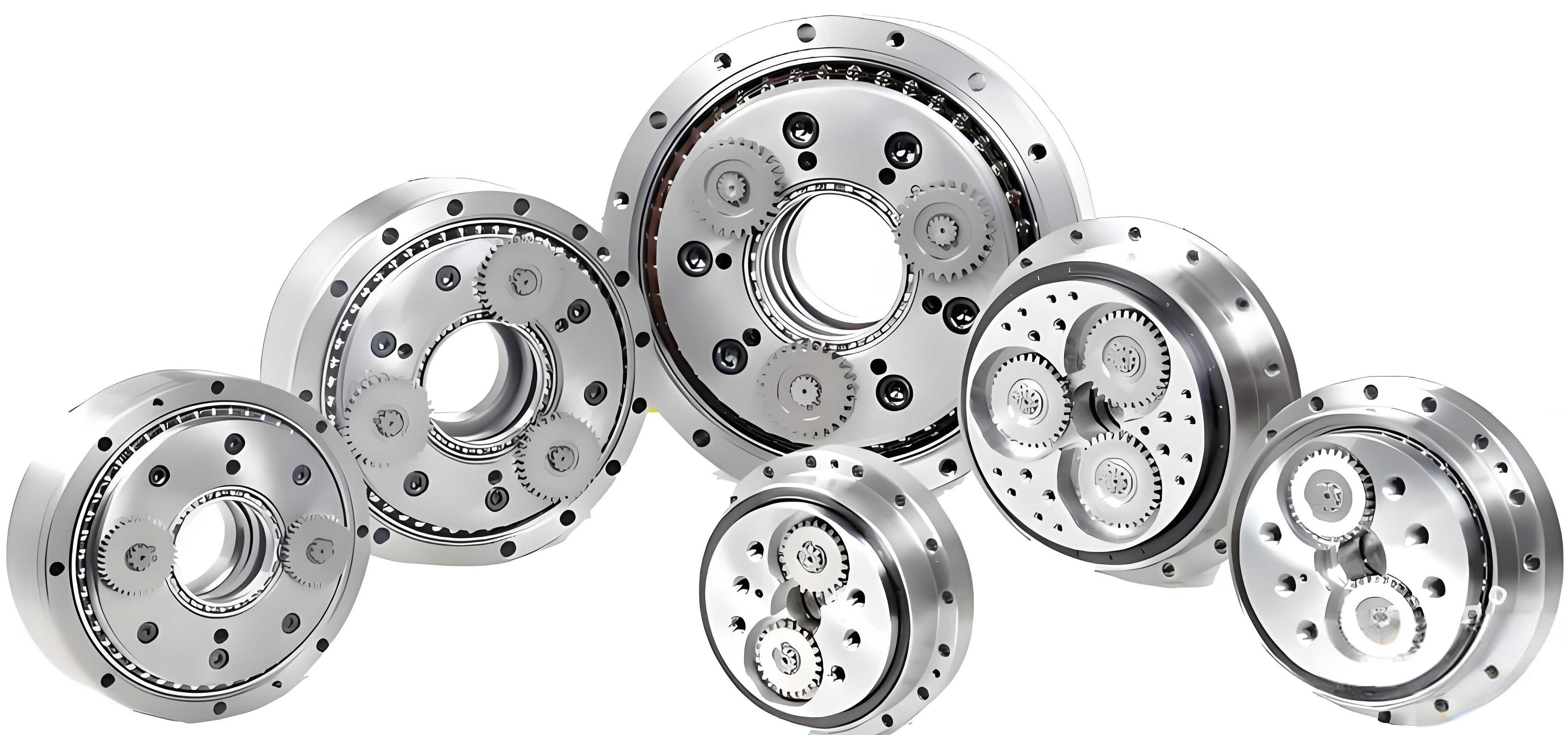
Rotary vector (RV) reducers are renowned for their high reduction ratios, compact size, substantial rigidity, superior motion accuracy, minimal backlash, high transmission efficiency, smooth operation, and strong load-bearing capacity. These characteristics make them indispensable in high-precision transmission fields such as industrial robot joints, CNC machine tools, and automated equipment. However, achieving this level of performance requires stringent control over transmission error, which is defined as the deviation of the actual output angle from its theoretical value under unidirectional input rotation. This error directly impacts the positioning accuracy and operational smoothness of the end effector. The domestic market for RV reducers has long been dominated by a few international companies, and controlling transmission error remains a significant hurdle for domestic production. While prior research has explored aspects of RV reducer accuracy using geometric methods, quality-spring equivalence models, and virtual prototyping simulations, a systematic analysis ranking the influence of multiple, simultaneously present error sources has been lacking. Our work addresses this gap by analyzing the combined effects of five critical error factors.
We established a detailed virtual prototype model of an RV-40E-81 type rotary vector reducer. The three-dimensional solid models of all components, including the sun gear, planetary gears, and cycloid gears, were created using Pro/ENGINEER software with parametric modeling techniques to facilitate easy modification of geometric parameters for subsequent experiments. The model was then imported into the ADAMS multi-body dynamics software in Parasolid format. Mass and material properties were assigned, and the assembly was simplified by omitting minor features like chamfers, bolts, and pins, which have negligible impact on the macro-level transmission error. The dynamic model incorporated 12 revolute joints and 82 contact pairs defined using the IMPACT function. The simulation was configured with a WSTIFF solver and SI2 integration format for accuracy. A step function was applied to the input shaft to ramp its rotational speed from 0 to 5700 deg/s within the first second, and the total simulation time was set to 6 seconds. The correctness of the virtual prototype was verified by comparing the input angular velocity profile with the expected reduced output angular velocity profile, confirming the model’s validity for transmission error analysis.
The core of our investigation utilizes the orthogonal experimental design method, a statistical technique for efficiently analyzing multi-factor problems using an “orthogonal array.” We focused on five primary error factors from the secondary cycloidal-pin gear transmission stage, which has a dominant influence on the overall error due to its high reduction ratio. The selected factors and their chosen levels, based on practical manufacturing considerations and sensitivity analysis, are presented in Table 1.
| Factor | A: Cycloid Isometric Modification (mm) | B: Cycloid Profile Shift Modification (mm) | C: Eccentricity Error (mm) | D: Pin Center Circle Radius Error (mm) | E: Pin Radius Error (mm) |
|---|---|---|---|---|---|
| Level 1 | -0.026 | -0.01 | 0.05 | 0.05 | 0.05 |
| Level 2 | -0.05 | 0.01 | 0.07 | 0.07 | 0.07 |
| Level 3 | 0.01 | 0.05 | 0.10 | 0.10 | 0.10 |
Considering the five factors at three levels each and including the potential interaction between Factors A and B (A×B), the total degrees of freedom required was 14. We selected the L27(3^13) orthogonal array, which has 26 degrees of freedom, to accommodate all factors and interactions. The complete experimental design matrix, assigning factors to specific columns of the orthogonal table, along with the simulated transmission error result for each combination, is shown in Table 2. The transmission error for each test was extracted from the ADAMS simulation output.
| Test No. | A | B | (A×B)1 | (A×B)2 | C | D | E | Transmission Error (arc-seconds) |
|---|---|---|---|---|---|---|---|---|
| 1 | 1 | 1 | 1 | 1 | 1 | 1 | 1 | 2.261 |
| 2 | 1 | 1 | 1 | 1 | 2 | 2 | 2 | 8.851 |
| 3 | 1 | 1 | 1 | 1 | 3 | 3 | 3 | 4.743 |
| 4 | 1 | 2 | 2 | 2 | 1 | 1 | 1 | 11.304 |
| 5 | 1 | 2 | 2 | 2 | 2 | 2 | 2 | 12.820 |
| 6 | 1 | 2 | 2 | 2 | 3 | 3 | 3 | 4.426 |
| 7 | 1 | 3 | 3 | 3 | 1 | 1 | 1 | 6.111 |
| 8 | 1 | 3 | 3 | 3 | 2 | 2 | 2 | 19.001 |
| 9 | 1 | 3 | 3 | 3 | 3 | 3 | 3 | 12.110 |
| 10 | 2 | 1 | 2 | 3 | 1 | 2 | 3 | 8.148 |
| 11 | 2 | 1 | 2 | 3 | 2 | 3 | 1 | 7.693 |
| 12 | 2 | 1 | 2 | 3 | 3 | 1 | 2 | 11.064 |
| 13 | 2 | 2 | 3 | 1 | 1 | 2 | 3 | 53.620 |
| 14 | 2 | 2 | 3 | 1 | 2 | 3 | 1 | 5.377 |
| 15 | 2 | 2 | 3 | 1 | 3 | 1 | 2 | 12.638 |
| 16 | 2 | 3 | 1 | 2 | 1 | 2 | 3 | 33.580 |
| 17 | 2 | 3 | 1 | 2 | 2 | 3 | 1 | 13.867 |
| 18 | 2 | 3 | 1 | 2 | 3 | 1 | 2 | 12.528 |
| 19 | 3 | 1 | 3 | 2 | 1 | 3 | 2 | 7.209 |
| 20 | 3 | 1 | 3 | 2 | 2 | 1 | 3 | 5.282 |
| 21 | 3 | 1 | 3 | 2 | 3 | 2 | 1 | 8.128 |
| 22 | 3 | 2 | 1 | 3 | 1 | 3 | 2 | 5.413 |
| 23 | 3 | 2 | 1 | 3 | 2 | 1 | 3 | 6.088 |
| 24 | 3 | 2 | 1 | 3 | 3 | 2 | 1 | 15.409 |
| 25 | 3 | 3 | 2 | 1 | 1 | 3 | 2 | 3.864 |
| 26 | 3 | 3 | 2 | 1 | 2 | 1 | 3 | 9.123 |
| 27 | 3 | 3 | 2 | 1 | 3 | 2 | 1 | 20.532 |
We performed both range analysis and variance analysis on the orthogonal experimental results. The range (R) for each factor, calculated as the difference between the maximum and minimum average effect at its three levels, provides an initial ranking of influence. The results of the range analysis, including the sum (K_i) and average (k_i) of results for each factor level, are summarized below, derived from Table 2. The total sum T of all transmission errors is 321.19 arc-seconds.
$$k_i = \frac{K_i}{s}$$
$$R = \max(k_1, k_2, k_3) – \min(k_1, k_2, k_3)$$
Where \( s \) is the number of times each level appears in a column (9 for L27). The calculated ranges were: R_A=8.608, R_B=7.482, R_C=4.823, R_D=12.821, R_E=5.465. This suggests Factor D (pin center circle radius error) has the largest effect, followed by A, B, E, and C.
For a more rigorous statistical evaluation, analysis of variance (ANOVA) was conducted. The total sum of squares (S_T), factor sum of squares (S_J), degrees of freedom (f), mean square (V_J), and the F-ratio (F_J) were calculated according to standard ANOVA procedures. The error mean square (V_e) was estimated from the empty columns in the orthogonal array. The ANOVA results are presented in Table 3.
| Variance Source | Sum of Squares (S) | Degrees of Freedom (f) | Mean Square (V) | F-ratio (F) |
|---|---|---|---|---|
| A (Isometric Mod.) | 441.231 | 2 | 220.6155 | 3.1594 |
| B (Profile Shift Mod.) | 318.782 | 2 | 159.3910 | 2.2826 |
| A×B (Interaction) | 144.877 | 4 | 36.2193 | 0.5187 |
| C (Eccentricity Error) | 109.696 | 2 | 54.8480 | 0.7855 |
| D (Pin Center Circle Error) | 896.392 | 2 | 448.1960 | 6.4185 |
| E (Pin Radius Error) | 150.974 | 2 | 75.4870 | 1.0810 |
| Error (e) | 837.940 | 12 | 69.8283 | – |
| Total (T) | 2899.892 | 26 | – | – |
Comparing the mean squares (V), the order of influence is confirmed as: D > A > B > E > C > (A×B). Significance testing was performed by comparing the calculated F-ratios against critical F-values at a significance level of α=0.1: F_{0.1}(2,12)=2.81 and F_{0.1}(4,12)=2.48. Since F_D = 6.4185 > 2.81 and F_A = 3.1594 > 2.81, Factors D and A are statistically significant. The F-ratios for other factors, including the interaction A×B, are below their respective critical values, indicating their effects are not statistically significant within the tested level ranges. This finding implies that, for this specific rotary vector reducer configuration, the interaction between isometric and profile shift modifications is negligible compared to the main effects.
The trend of transmission error variation with each factor level can be visualized. For the isometric modification (A), error increases when moving from -0.026 mm to -0.05 mm, then decreases sharply when transitioning to a positive modification of +0.01 mm. For profile shift (B), error increases steadily from negative to positive shift. Eccentricity error (C) shows a complex trend: error decreases slightly from 0.05 mm to 0.07 mm, then increases again at 0.10 mm. Pin center circle radius error (D) causes error to increase dramatically from 0.05 mm to 0.07 mm, followed by a decrease at 0.10 mm. Pin radius error (E) leads to a gradual, then sharper, increase in error across its level range. These non-linear trends highlight the complexity of error interactions within the rotary vector reducer mechanism.
Based on the analysis, the optimal combination of factor levels that minimizes transmission error is identified as A3B1C2D3E1. This corresponds to an isometric modification of +0.01 mm, a profile shift of -0.01 mm, an eccentricity error of 0.07 mm, a pin center circle radius error of 0.10 mm, and a pin radius error of 0.05 mm. It is crucial to note that this “optimal” combination is derived within the constraints of the chosen discrete levels and may represent a local minimum. Furthermore, some error values (like 0.10 mm for pin center circle) are relatively large; in practice, minimizing all errors is desirable, and the hierarchy (D being most critical) is the key practical insight.
To establish a theoretical foundation, we derived individual formulas for the transmission error contribution (\(\Delta \phi_i\)) from each of the four main manufacturing errors (excluding interaction), based on the kinematics of the cycloidal drive. For a rotary vector reducer with pin number \(z_c\), crank eccentricity \(a\), and a design parameter \(K_1 = \frac{a z_c}{r_{rp}}\) (where \(r_{rp}\) is the pin center circle radius), the contributions are:
Contribution from cycloid gear modifications (isometric \(\Delta r_{rp}\), profile shift \(\Delta r_p\)):
$$\Delta \phi_1 = \frac{180 \times 60}{\pi} \times \left( \frac{2 \Delta r_{rp}}{a z_c} – \frac{2 \Delta r_p}{a z_c \sqrt{1-K_1^2}} \right)$$
Contribution from eccentricity error (\(\delta a\)):
$$\Delta \phi_2 = \frac{180 \times 60}{\pi} \times \left( -2 k_n \delta a \right)$$
where \(k_n\) is a transmission ratio related constant.
Contribution from pin center circle radius error (\(\delta r_{rp}\)):
$$\Delta \phi_3 = \frac{180 \times 60}{\pi} \times \frac{2 \delta r_{rp} \sqrt{1-K_1^2}}{a z_c}$$
Contribution from pin radius error (\(\delta r_{rp}’\)):
$$\Delta \phi_4 = \frac{180 \times 60}{\pi} \times \left( -\frac{2}{a z_c} \delta r_{rp}’ \right)$$
The theoretical total transmission error, assuming linear superposition, is:
$$\Delta \phi_{\Sigma} = \Delta \phi_1 + \Delta \phi_2 + \Delta \phi_3 + \Delta \phi_4$$
Substituting the parameters for the RV-40E model and the optimal error values (A3B1C2D3E1) into these equations yields a theoretical transmission error of \( \Delta \phi_{\Sigma (theory)} \approx 1.5179 \) arc-seconds. This linear model provides a baseline but does not account for non-linear interactions between errors.
To capture the non-linear relationships evident in the orthogonal experiment results, we developed a more accurate empirical model using a second-order multivariate regression. The general form of the model for \(m\) factors is:
$$y = a + \sum_{j=1}^{m} b_j x_j + \sum_{j=1}^{m} b_{jj} x_j^2 + \sum_{j < k} b_{jk} x_j x_k$$
For our five factors (A, B, C, D, E), the full model includes linear, quadratic, and two-way interaction terms. Using the data from Table 2 and MATLAB’s regression tools, we performed the analysis. Two data points (Tests 10 and 13) were identified as outliers and removed to improve model robustness. The resulting regression formula for transmission error \(y\) (in arc-seconds) is:
$$
\begin{aligned}
y = & -96.8567 – 1866.4088x_1 – 13.1091x_2 + 1100.6656x_3 + 913.6743x_4 + 242.8159x_5 \\
& -1791.8425x_1^2 – 668.0729x_2^2 + 359.1942x_1x_2 + 16969.6831x_1x_3 + 2363.2887x_2x_3 \\
& + 5271.5643x_1x_4 + 334.5837x_2x_4 – 11308.2223x_3x_4 – 1015.6731x_2x_5
\end{aligned}
$$
Where \(x_1\) is isometric modification (mm), \(x_2\) is profile shift (mm), \(x_3\) is eccentricity error (mm), \(x_4\) is pin center circle radius error (mm), and \(x_5\) is pin radius error (mm). The model’s goodness-of-fit is indicated by a coefficient of determination \(r^2 = 0.89\), an F-statistic of 5.66, and a corresponding p-value of 0.004, which is less than the significance level of 0.05. This confirms the regression model is statistically significant and provides a reliable fit to the experimental data.
To validate our findings, we performed a final simulation using the virtual prototype configured with the optimal error combination A3B1C2D3E1. The resulting transmission error curve was analyzed. The peak-to-peak transmission error, calculated as \( |y_{max}| + |y_{min}| \) from the stable simulation period, was found to be approximately 1.4424 arc-seconds. This simulation result serves as our benchmark.
We then compared this benchmark against the predictions from our two models. The theoretical linear superposition model predicted 1.5179 arc-seconds, resulting in an error of about 5.23% relative to the simulation. The non-linear regression model predicted 1.3949 arc-seconds, resulting in a smaller error of about 3.29%. This comparison demonstrates two key points: first, the linear theoretical model provides a reasonable estimate but over-predicts error, likely because it sums individual contributions without considering potential error cancellations within the assembled rotary vector reducer. Second, the non-linear regression model, derived directly from the orthogonal experiment data, offers a more accurate and reliable prediction tool. Its accuracy, combined with its ability to accept any combination of error values within the studied ranges (not just the discrete levels from the experiment), makes it a highly practical formula for estimating the transmission error of this type of rotary vector reducer during the design and tolerance specification phase.
In conclusion, our integrated approach of virtual prototyping and orthogonal experiment design has successfully elucidated the complex relationships between manufacturing errors and transmission accuracy in an RV reducer. The primary findings are: Firstly, among the factors studied, the pin center circle radius error has the most significant and pronounced influence on the overall transmission error of the rotary vector reducer. The isometric modification of the cycloid gear also shows a statistically significant effect. Secondly, the eccentricity error exhibits the smallest influence within the tested ranges, and the interaction between the two cycloid gear modification types is negligible. Thirdly, the trends between each error factor and the transmission error are predominantly non-linear, underscoring the complexity of the system. Finally, the second-order multivariate regression model we developed provides a computationally efficient and sufficiently accurate method for estimating transmission error based on specified component errors, offering a valuable tool for engineers in the design and tolerance analysis of rotary vector reducers. This work contributes to a deeper understanding of accuracy control in RV reducers, supporting progress towards higher performance and domestic manufacturing capabilities.