
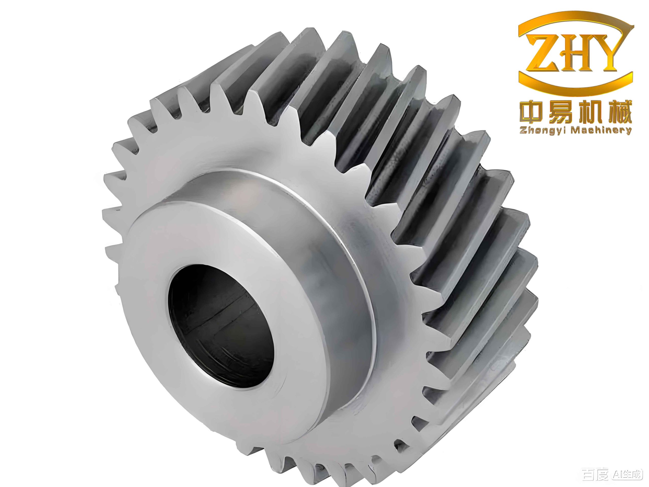
I have investigated a design method for high power density asymmetric helical gears used in electric vehicle transmissions. The central problem is straightforward: electric vehicles require reducers that transmit larger torque within a smaller installation space, while maintaining distinct durability requirements for forward driving and forward reverse dragging. Conventional symmetric involute helical gears use the same pressure angle on both flanks, so increasing the pressure angle to raise load capacity also thins the tooth tip and can worsen tip fracture risk. Asymmetric helical gears solve this conflict by assigning different pressure angles to the driving flank and the coast flank. In my work, I combine tooth surface generation, geometric tooth contact analysis, loaded tooth contact analysis, macro geometry optimization, and micro modification optimization to obtain asymmetric helical gears with higher power density and smoother meshing behavior.
1. Design Motivation and Asymmetric Principle
In an electric vehicle reducer, the driving flank usually operates under acceleration and continuous traction, whereas the coast flank mainly operates during regenerative braking and reverse drag. Field experience and standard durability specifications indicate that the driving direction demands a longer fatigue life than the reverse-drag direction. Therefore, the two flanks of a gear tooth should not be treated identically. I use a larger pressure angle on the driving flank to reduce contact stress and a smaller pressure angle on the coast flank to preserve tip thickness. This arrangement allows the gear pair to carry higher torque without increasing the outer dimensions. The resulting asymmetric helical gears can therefore improve the power-to-volume ratio of the reducer.
For a symmetric helical gear pair, the contact stress and root bending stress are controlled mainly by the normal module, helix angle, tooth number, and pressure angle. Increasing the pressure angle reduces contact stress but increases the radial force. Increasing the module reduces both contact and bending stresses but increases the center distance. Increasing the helix angle reduces stress through higher contact ratio but also increases axial force and may enlarge the gearbox. My design approach treats these variables as a coupled optimization problem rather than a set of independent selections.
2. Mathematical Model of Asymmetric Helical Gears
I generate the asymmetric helical gear tooth surface from a rack cutter with two different pressure angles. The rack cutter profile is divided into a left involute segment, a right involute segment, and two fillet arcs. The left flank corresponds to the driving side, and the right flank corresponds to the coast side. Let \(j=1\) denote the driving flank and \(j=2\) denote the coast flank. The position vector of the rack cutter in its local coordinate system is written as
$$ \mathbf{R}_{j}(l_j,u_j) = \begin{bmatrix} x_j \\ y_j \\ z_j \\ 1 \end{bmatrix} = \begin{bmatrix} l_j \\ 0 \\ u_j \\ 1 \end{bmatrix} $$
where \(l_j\) and \(u_j\) are independent parameters along the profile and the axial direction, respectively. The transformation from the local cutter coordinate system to the rack coordinate system is performed by
$$ \mathbf{R}_{bj}(l_j,u_j) = \mathbf{M}_{bj} \mathbf{R}_{j}(l_j,u_j) $$
where \(\mathbf{M}_{bj}\) is the homogeneous transformation matrix. The unit normal vector of the rack cutter surface is obtained from the cross product of the two tangent vectors:
$$ \mathbf{n}_{bj} = \frac{\partial \mathbf{R}_{bj}}{\partial l_j} \times \frac{\partial \mathbf{R}_{bj}}{\partial u_j} \Big/ \left\| \frac{\partial \mathbf{R}_{bj}}{\partial l_j} \times \frac{\partial \mathbf{R}_{bj}}{\partial u_j} \right\| $$
For the fillet arcs, the position vector is expressed using the arc center and the arc angle. I write the fillet arc in the cutter coordinate system as
$$ \mathbf{R}_{sj}(\varphi_j,u_j) = \begin{bmatrix} X_{0j} – \rho \cos\varphi_j \\ Y_{0j} – \rho \sin\varphi_j \\ u_j \\ 1 \end{bmatrix} $$
where \(X_{0j}\) and \(Y_{0j}\) are the coordinates of the arc center, \(\rho\) is the fillet radius, and \(\varphi_j\) is the arc parameter. The normal vector is obtained in the same way as for the involute segment. During generation, the rack cutter translates and the gear rotates. The meshing equation between the rack cutter and the gear tooth surface is
$$ f_i = \mathbf{n}_{bj} \cdot \mathbf{v}^{(12)} = 0 $$
where \(\mathbf{v}^{(12)}\) is the relative velocity between the cutter and the gear at the contact point. Solving this equation together with the coordinate transformation yields the generated tooth surface. For the involute portion, I obtain
$$ \mathbf{R}_{i}(l_j,u_j,\theta) = \mathbf{M}_{ib} \mathbf{R}_{bj}(l_j,u_j) $$
$$ \mathbf{n}_{i}(l_j,u_j,\theta) = \mathbf{L}_{ib} \mathbf{n}_{bj}(l_j,u_j) $$
where \(\theta\) is the gear rotation angle, \(\mathbf{M}_{ib}\) is the transformation matrix from the rack coordinate system to the gear coordinate system, and \(\mathbf{L}_{ib}\) is the corresponding direction transformation matrix. For the fillet portion, the generated surface satisfies
$$ \mathbf{R}_{is}(u_j,\varphi_j,\theta) = \mathbf{M}_{if} \mathbf{R}_{fsj}(u_j,\varphi_j,\theta) $$
$$ f_{sj} = \mathbf{n}_{fsj} \cdot \mathbf{v}^{(12)} = 0 $$
By assembling the involute and fillet surfaces, I obtain a complete asymmetric helical gear tooth surface. The input parameters include the normal module \(m_n\), tooth numbers \(z_1\) and \(z_2\), driving pressure angle \(\alpha_{n1}\), coast pressure angle \(\alpha_{n2}\), helix angle \(\beta\), tooth width \(b\), addendum \(h_a\), dedendum \(h_f\), fillet radius \(\rho\), and profile shift coefficients \(x_{n1}\) and \(x_{n2}\). This model provides high geometric accuracy for both flanks of the asymmetric helical gears.
3. Tooth Contact Analysis and Loaded Tooth Contact Analysis
After generating the tooth surfaces, I establish a geometric tooth contact analysis model. The two gear surfaces must have a common contact point and a common normal at every instant. In a fixed coordinate system, the contact conditions are
$$ \mathbf{R}_{f}^{(1)}(u_1,l_1,\phi_1) = \mathbf{R}_{f}^{(2)}(u_2,l_2,\phi_2) $$
$$ \mathbf{n}_{f}^{(1)}(u_1,l_1,\phi_1) = \mathbf{n}_{f}^{(2)}(u_2,l_2,\phi_2) $$
where \(\phi_1\) and \(\phi_2\) are the rotation angles of the driving and driven gears. Because the normal vectors are unit vectors, the above vector equations provide five independent scalar equations. By specifying a sequence of driving gear rotation angles, I solve for the remaining unknowns and obtain the contact path. The geometric transmission error is computed as
$$ \Delta\phi_2 = (\phi_2 – \phi_{20}) – \frac{z_1}{z_2}(\phi_1 – \phi_{10}) $$
I also analyze the sensitivity of asymmetric helical gears to installation errors. The installation errors include the horizontal axis error \(\Delta\delta\) and the vertical axis error \(\Delta\varepsilon\). A larger allowable error range means better tolerance. I evaluated the contact pattern under different pressure angles and found that a larger driving pressure angle generally improves tolerance to installation errors. The results are summarized in Table 1.
| Driving pressure angle \(\alpha_{n1}\) / ° | Error type | Allowable range | Total tolerance |
|---|---|---|---|
| 15 | \(\Delta\delta\) / ° | [-0.042, 0.044] | 0.086 |
| 15 | \(\Delta\varepsilon\) / ° | [-0.013, 0.012] | 0.025 |
| 17.5 | \(\Delta\delta\) / ° | [-0.048, 0.045] | 0.093 |
| 17.5 | \(\Delta\varepsilon\) / ° | [-0.016, 0.015] | 0.031 |
| 20 | \(\Delta\delta\) / ° | [-0.044, 0.047] | 0.092 |
| 20 | \(\Delta\varepsilon\) / ° | [-0.019, 0.018] | 0.037 |
| 22.5 | \(\Delta\delta\) / ° | [-0.052, 0.049] | 0.101 |
| 22.5 | \(\Delta\varepsilon\) / ° | [-0.025, 0.021] | 0.046 |
| 25 | \(\Delta\delta\) / ° | [-0.051, 0.050] | 0.101 |
| 25 | \(\Delta\varepsilon\) / ° | [-0.025, 0.025] | 0.050 |
For loaded tooth contact analysis, I use the flexibility matrix of the gear teeth and the contact compatibility condition. The loaded contact model is governed by
$$ \mathbf{F}\mathbf{p} + \mathbf{w} + \mathbf{d} = \mathbf{Z} $$
where \(\mathbf{F}\) is the normal flexibility matrix, \(\mathbf{p}\) is the normal load vector, \(\mathbf{w}\) is the initial contact gap vector, \(\mathbf{d}\) is the residual gap vector, and \(\mathbf{Z}\) is the normal displacement vector. The force equilibrium condition is
$$ \sum_{q=1}^{n} p_q = P $$
The contact condition requires that the load is positive only where the gap vanishes. This leads to the following mathematical programming model:
$$ \min \left( \frac{1}{2} \mathbf{p}^T \mathbf{F} \mathbf{p} + \mathbf{w}^T \mathbf{p} \right) $$
$$ \text{subject to } \mathbf{F}\mathbf{p} + \mathbf{w} + \mathbf{d} = \mathbf{Z}, \quad \mathbf{p} \ge 0, \quad \mathbf{d} \ge 0, \quad \mathbf{p}^T \mathbf{d} = 0 $$
After solving this model, I obtain the load distribution along the contact line. The maximum contact stress at the center of the contact ellipse is calculated by
$$ \sigma_H = \frac{3P}{2\pi a_c b_c} $$
where \(a_c\) and \(b_c\) are the semi-major and semi-minor axes of the contact ellipse. These axes are determined from the principal curvatures and the elastic properties of the materials:
$$ a_c = \left( \frac{3P}{4A_c} \left( \frac{1-\mu_1^2}{E_1} + \frac{1-\mu_2^2}{E_2} \right) \right)^{1/3} $$
$$ b_c = \left( \frac{3P}{4B_c} \left( \frac{1-\mu_1^2}{E_1} + \frac{1-\mu_2^2}{E_2} \right) \right)^{1/3} $$
The root bending stress is obtained by using an influence matrix \(\mathbf{S}\) and the load vector \(\mathbf{L}\):
$$ \boldsymbol{\sigma}_F = \mathbf{S}\mathbf{L} $$
Using these formulations, I can evaluate the contact stress and bending stress of asymmetric helical gears under torque. The analysis shows that the contact stress increases with load, and the bending stress also increases with load. The load distribution is affected by installation errors, especially the horizontal axis error.
4. Macro Geometry Optimization for High Power Density
I performed a systematic study of how macro geometry parameters influence the stresses in asymmetric helical gears. The driving pressure angle \(\alpha_{n1}\), coast pressure angle \(\alpha_{n2}\), normal module \(m_n\), helix angle \(\beta\), and tooth numbers \(z_1\) and \(z_2\) were considered. The key findings are summarized in Table 2 for bending stress and Table 3 for contact stress.
| Driving pressure angle \(\alpha_{n1}\) / ° | Coast pressure angle \(\alpha_{n2}\) / ° | Driving gear bending stress / MPa | Driven gear bending stress / MPa |
|---|---|---|---|
| 17.5 | 15 | 383 | 374 |
| 17.5 | 20 | 340.3 | 326.9 |
| 17.5 | 25 | 314.4 | 294.4 |
| 20 | 15 | 413.9 | 425.1 |
| 20 | 20 | 376.5 | 355.3 |
| 20 | 25 | 348.4 | 331.7 |
| 22.5 | 15 | 439 | 495.4 |
| 22.5 | 20 | 391.4 | 427.1 |
| 22.5 | 25 | 360.3 | 389.6 |
Table 2 shows that increasing the coast pressure angle reduces the bending stress on both gears. When the coast pressure angle is fixed, increasing the driving pressure angle increases the bending stress. This means that a larger driving pressure angle improves contact stress but may reduce bending strength. Therefore, the two pressure angles must be selected together.
| Driving pressure angle \(\alpha_{n1}\) / ° | Contact stress for \(\alpha_{n2}=15^\circ\) / MPa | Contact stress for \(\alpha_{n2}=20^\circ\) / MPa | Contact stress for \(\alpha_{n2}=25^\circ\) / MPa |
|---|---|---|---|
| 17.5 | 1829 | 1828 | 1827 |
| 20 | 1342 | 1342 | 1347 |
| 22.5 | 1146 | 1147 | 1150 |
Table 3 shows that the contact stress is controlled mainly by the driving pressure angle. Increasing the driving pressure angle from 17.5° to 22.5° reduces the contact stress from about 1828 MPa to about 1147 MPa. The coast pressure angle has only a minor effect on contact stress. This confirms that the driving flank should use a larger pressure angle for high load capacity.
The influence of the normal module on contact stress is shown in Table 4. A larger module reduces contact stress because the tooth becomes thicker and the radius of curvature increases. However, a larger module also increases the center distance and gear volume.
| Normal module \(m_n\) / mm | Contact stress for \(\alpha_{n1}/\alpha_{n2}=20^\circ/20^\circ\) / MPa | Contact stress for \(\alpha_{n1}/\alpha_{n2}=22.5^\circ/20^\circ\) / MPa |
|---|---|---|
| 1.5 | 2129.3 | 1432.4 |
| 1.75 | 1487.9 | 1230.8 |
| 2.0 | 1244.8 | 1066.4 |
| 2.25 | 1074.1 | 934.3 |
| 2.5 | 973.3 | 844.5 |
I also found that increasing the helix angle reduces both contact stress and bending stress because the contact ratio increases. Increasing the pinion tooth number reduces stress because the pinion diameter increases, but it also increases the center distance. Therefore, the optimization must balance load capacity and volume.
I constructed a high power density optimization model. The objective was to minimize the center distance while satisfying stress, tip thickness, and undercut constraints. The optimization variables were the driving pressure angle, coast pressure angle, pinion tooth number, gear tooth number, normal module, and helix angle:
$$ \mathbf{X} = \begin{bmatrix} \alpha_{n1} & \alpha_{n2} & z_1 & z_2 & m_n & \beta \end{bmatrix}^T $$
The optimization problem was formulated as
$$ \min_{\mathbf{X}} \left( \frac{E_{P0}}{E_P} \right) $$
where \(E_{P0}\) is the power density of the baseline symmetric gear pair and \(E_P\) is the power density of the optimized asymmetric gear pair. The power density is defined as the transmitted power per unit volume:
$$ E_P = \frac{P}{V} = \frac{2 \pi n T}{60 V} $$
where \(T\) is the torque, \(n\) is the rotational speed, and \(V\) is the volume of the gear pair. The constraints include
$$ \sigma_{H1} \le \sigma_{HP1}, \quad \sigma_{H2} \le \sigma_{HP2} $$
$$ \sigma_{F1} \le \sigma_{FP1}, \quad \sigma_{F2} \le \sigma_{FP2} $$
$$ S_{a1} \ge 0.4 m_n, \quad S_{a2} \ge 0.4 m_n $$
$$ g_1 \ge 0, \quad g_2 \ge 0 $$
$$ 20^\circ \le \alpha_{n1} \le 24^\circ, \quad 16^\circ \le \alpha_{n2} \le 20^\circ $$
$$ 1.5 \le m_n \le 2.5, \quad 20^\circ \le \beta \le 30^\circ $$
Here \(\sigma_{H}\) and \(\sigma_{F}\) are contact and bending stresses, \(\sigma_{HP}\) and \(\sigma_{FP}\) are allowable stresses, and \(g_1\) and \(g_2\) are undercut prevention conditions. I used a genetic algorithm to solve this nonlinear optimization problem. The genetic algorithm parameters were set as follows: population size 20, crossover probability 0.9, mutation probability 0.05, and maximum generation 60. The optimization flow is summarized as:
$$ \text{Initialize population} \rightarrow \text{Evaluate TCA and LTCA} \rightarrow \text{Compute fitness} \rightarrow \text{Select, crossover, mutate} \rightarrow \text{Check convergence} $$
The optimized parameters and the comparison with the baseline symmetric helical gears are given in Table 5.
| Parameter | Baseline symmetric helical gears | Optimized asymmetric helical gears |
|---|---|---|
| Pinion tooth number \(z_1\) | 26 | 23 |
| Gear tooth number \(z_2\) | 75 | 69 |
| Normal module \(m_n\) / mm | 1.88 | 1.944 |
| Driving pressure angle \(\alpha_{n1}\) / ° | 20 | 21.483 |
| Coast pressure angle \(\alpha_{n2}\) / ° | 20 | 18.855 |
| Helix angle \(\beta\) / ° | 21.5 | 23.85 |
| Power density / (kW/m³) | 41464 | 44656 |
The optimization increased the power density by 7.65 %. The driving flank contact stress decreased by 12.29 %, the driving flank pinion bending stress decreased by 6.53 %, and the coast flank contact stress increased by 9.25 %. All stresses remained within allowable limits. This confirms that asymmetric helical gears are better suited to the different life requirements of forward driving and reverse dragging. The optimized asymmetric helical gears therefore achieve higher power density without sacrificing reliability.
5. Micro Modification Optimization for Vibration Reduction
High rotational speeds in electric vehicle reducers make loaded transmission error a dominant excitation for vibration and noise. I proposed a three-dimensional topological modification method for the driving pinion of asymmetric helical gears. The modification curve consists of a straight middle segment and parabolic end segments. The profile modification curve is
$$ \delta_p(h) = \begin{cases} l_1 \left( \frac{h – r_h}{l_3} \right)^2, & r_h \le h \le r_h + l_3 \\ 0, & r_h + l_3 < h < r_a – l_4 \\ l_2 \left( \frac{h – r_a}{l_4} \right)^2, & r_a – l_4 \le h \le r_a \end{cases} $$
The lead modification curve is
$$ \delta_t(l) = \begin{cases} l_5 \left( \frac{l + b/2}{l_7} \right)^2, & -\frac{b}{2} \le l \le -\frac{b}{2} + l_7 \\ 0, & -\frac{b}{2} + l_7 < l < \frac{b}{2} – l_7 \\ l_6 \left( \frac{l – b/2}{l_7} \right)^2, & \frac{b}{2} – l_7 \le l \le \frac{b}{2} \end{cases} $$
where \(l_1\) and \(l_2\) are the root and tip modification depths, \(l_3\) and \(l_4\) are the corresponding modification lengths, \(l_5\) and \(l_6\) are the left and right lead modification depths, and \(l_7\) is the unmodified lead length. The total modification amount at a point \((h,l)\) is
$$ \delta(h,l) = \delta_p(h) + \delta_t(l) $$
The modified pinion tooth surface is obtained by superimposing the modification surface on the theoretical surface:
$$ \mathbf{R}_r'(u_1,l_1) = \mathbf{R}_r(u_1,l_1) + \delta(h,l) \mathbf{n}_r(u_1,l_1) $$
I analyzed the influence of profile modification, lead modification, and topological modification on the loaded transmission error. The results show that root relief reduces the transmission error fluctuation when the pinion leaves meshing, while tip relief reduces the fluctuation when the pinion enters meshing. Excessive modification increases the fluctuation. Lead modification at the left or right end can remove edge contact, but it may increase the transmission error if applied alone. Topological modification combines the advantages of both and produces a smoother transmission error curve.
I then formulated an optimization problem to minimize the loaded transmission error fluctuation amplitude. The optimization variables were the seven modification parameters:
$$ \mathbf{l} = \begin{bmatrix} l_1 & l_2 & l_3 & l_4 & l_5 & l_6 & l_7 \end{bmatrix} $$
The objective function was
$$ \min F(\mathbf{l}) = \omega_1 \left| f_1(\mathbf{l}) – f_{10} \right| + \omega_2 \left| f_2(\mathbf{l}) – f_{20} \right| $$
where \(f_1\) and \(f_2\) are the loaded transmission error fluctuation amplitudes at two torque levels, \(f_{10}\) and \(f_{20}\) are the corresponding values before modification, and \(\omega_1\) and \(\omega_2\) are weight factors. I set \(\omega_1 = \omega_2 = 0.5\). The constraints were
$$ 0 \le l_1 \le 10\,\mu\text{m}, \quad 0 \le l_2 \le 10\,\mu\text{m} $$
$$ 0 \le l_3 \le 2\,\text{mm}, \quad 0 \le l_4 \le 2\,\text{mm} $$
$$ 1 \le l_5 \le 10\,\mu\text{m}, \quad 1 \le l_6 \le 10\,\mu\text{m} $$
$$ 0 \le l_7 \le 15\,\text{mm} $$
The genetic algorithm produced the optimized modification parameters shown in Table 6.
| Parameter | Optimized value |
|---|---|
| Root modification depth \(l_1\) | 1.41 μm |
| Root modification length \(l_3\) | 0.043 mm |
| Tip modification depth \(l_2\) | 0.88 μm |
| Tip modification length \(l_4\) | 0.66 mm |
| Left lead modification depth \(l_5\) | 8.49 μm |
| Right lead modification depth \(l_6\) | 5.41 μm |
| Unmodified lead length \(l_7\) | 1.98 mm |
After optimization, the loaded transmission error fluctuation amplitude decreased from \(5.1\,\mu\text{m}\) to \(4.09\,\mu\text{m}\), a reduction of 19.8 %. The contact trace moved toward the middle of the tooth profile, and edge contact disappeared. The contact pattern became more uniform along the tooth width. These improvements indicate that topological modification is effective for reducing vibration excitation in asymmetric helical gears.
6. Verification of the Optimized Asymmetric Helical Gears
I verified the theoretical models using a professional gear transmission simulation software. The geometric parameters of the optimized asymmetric helical gears are listed in Table 7. The driving pinion modification parameters are those given in Table 6.
| Parameter | Pinion | Gear |
|---|---|---|
| Tooth number | 23 | 69 |
| Normal module \(m_n\) / mm | 1.944 | 1.944 |
| Driving pressure angle \(\alpha_{n1}\) / ° | 21.483 | 21.483 |
| Coast pressure angle \(\alpha_{n2}\) / ° | 18.855 | 18.855 |
| Helix angle \(\beta\) / ° | 23.85 | 23.85 |
| Addendum \(h_a\) / mm | 1.944 | 1.944 |
| Dedendum \(h_f\) / mm | 2.43 | 2.43 |
| Tooth width \(b\) / mm | 30 | 30 |
| Profile shift coefficient \(x_n\) | 0.051 | -0.062 |
I compared the contact stress and bending stress from my theoretical model with the simulation results. The comparison is shown in Table 8.
| Item | Theoretical result / MPa | Simulation result / MPa | Difference / % |
|---|---|---|---|
| Contact stress before optimization | 1177.1 | 1410 | 19.78 |
| Contact stress after optimization | 1215.9 | 1408.5 | 15.84 |
| Pinion bending stress before optimization | 351.9 | 374.4 | 6.39 |
| Pinion bending stress after optimization | 385.1 | 367.7 | 4.52 |
| Gear bending stress before optimization | 355.9 | 308.9 | 13.21 |
| Gear bending stress after optimization | 382.5 | 323.3 | 15.48 |
The differences between the theoretical and simulation results are within acceptable engineering accuracy. The trends of the bending stress curves also match well. I compared the geometric contact patterns before and after modification. Before modification, edge contact occurred at the tooth ends due to installation errors. After topological modification, the contact pattern moved to the middle of the tooth surface. The simulation results agreed with my tooth contact analysis. I also compared the loaded transmission error before and after modification. The theoretical curve and the simulation curve followed the same trend. The fluctuation amplitude decreased after modification. These comparisons validate the macro geometry optimization and the micro modification optimization methods for asymmetric helical gears.
7. Conclusions and Future Work
I developed a complete design method for high power density asymmetric helical gears in electric vehicle transmissions. The main conclusions are as follows.
First, I established a high-precision tooth surface model for asymmetric helical gears generated by a double-pressure-angle rack cutter. The model includes the involute flanks and the fillet arcs. I derived the geometric tooth contact analysis equations and the loaded tooth contact analysis equations. The installation error tolerance analysis showed that a larger driving pressure angle improves tolerance to horizontal and vertical axis errors.
Second, I analyzed the influence of macro geometry parameters on contact stress and bending stress. Increasing the driving pressure angle reduces contact stress but increases bending stress. Increasing the coast pressure angle reduces bending stress. Increasing the module, helix angle, or pinion tooth number reduces stresses but increases volume. I formulated a high power density optimization model and solved it with a genetic algorithm. The optimized asymmetric helical gears increased the power density by 7.65 % compared with symmetric helical gears.
Third, I proposed a three-dimensional topological modification method for the driving pinion. The modification curve consists of parabolic end segments and a straight middle segment. I analyzed the effects of profile modification, lead modification, and topological modification on loaded transmission error. The topological modification produced the smoothest transmission error curve. I optimized the modification parameters using a genetic algorithm. The loaded transmission error fluctuation amplitude decreased by 19.8 %. Edge contact disappeared, and the contact trace moved to the middle of the tooth profile.
Fourth, I verified the theoretical models with a professional gear simulation software. The contact stress, bending stress, contact pattern, and loaded transmission error from the theoretical model agreed with the simulation results within engineering accuracy. This verification supports the reliability of the proposed design method.
For future work, I plan to extend the dynamic model of asymmetric helical gears to include system-level coupling effects. I also intend to consider lubrication and cooling effects in the fatigue life calculation. These factors may allow even higher power density. Experimental validation on a test rig will also be performed to further confirm the theoretical predictions. I believe that asymmetric helical gears are a promising solution for electric vehicle reducers because they match the different durability requirements of driving and reverse dragging while improving power density and reducing vibration.