
I investigate the automatic monitoring of the operating state of drive pinion gears in drum-type rotary filter screens when multiple data sources are fused. The pinion gears in such a system are not isolated mechanical components. They operate under continuously changing load, speed, lubrication, alignment, and environmental conditions. When I examine a drum-type rotary filter screen, I see that the drive pinion gears engage a large ring gear, and the entire transmission chain is exposed to torque pulsation, debris, water flow disturbance, and varying resistance. A single vibration sensor or a single current sensor can reveal only part of this behavior. Therefore, I construct a monitoring framework in which vibration signals and current signals are fused, and I use a state-space representation to describe the hidden condition of the pinion gears. The hidden state is then estimated recursively by a Kalman filter. The result is an automatic monitoring method that produces precise operating information for the pinion gears and suppresses the information-island limitation of single-source monitoring.
The operating state of pinion gears has multidimensional features. If I rely only on vibration amplitude, I may confuse load variation with tooth surface degradation. If I rely only on motor current, I may detect a load change but fail to distinguish a local tooth defect from a global transmission resistance. For this reason, I treat vibration and current as complementary observations. Vibration reflects the mechanical response of the pinion gears, the ring gear, bearings, and shafts. Current reflects the electromagnetic torque and the load demanded by the drum and the pinion gears. When these two sources are combined, the observable space becomes richer, and the hidden state of the pinion gears can be estimated with lower uncertainty. I therefore define the monitoring problem as a joint state estimation problem rather than a threshold comparison problem.
In my method, the term pinion gears refers to the small driving gears that transmit motion to the large ring gear of the rotary filter screen. The pinion gears are repeatedly stressed during each revolution. Their contact pattern changes with load, misalignment, backlash, and lubrication. I model these effects through a state vector that includes representative variables such as contact severity, load torque, transmission error, and thermal or friction-related drift. The observations include vibration features in both the time domain and the frequency domain, as well as current features that indicate load variation. The mapping between the hidden state and the observations is defined by matrices that I estimate from normal and degraded operating data. The Kalman filter then predicts and updates the state of the pinion gears in real time.
I organize the remainder of this article around the construction of the state-space model, the extraction of multi-source features, the recursive estimation of the pinion gears state, the experimental configuration, and the performance evaluation. I use tables and equations throughout to make the parameterization explicit. The main objective is to show that multi-source fusion under a state-space formulation improves the reliability of automatic monitoring for pinion gears in drum-type rotary filter screens.
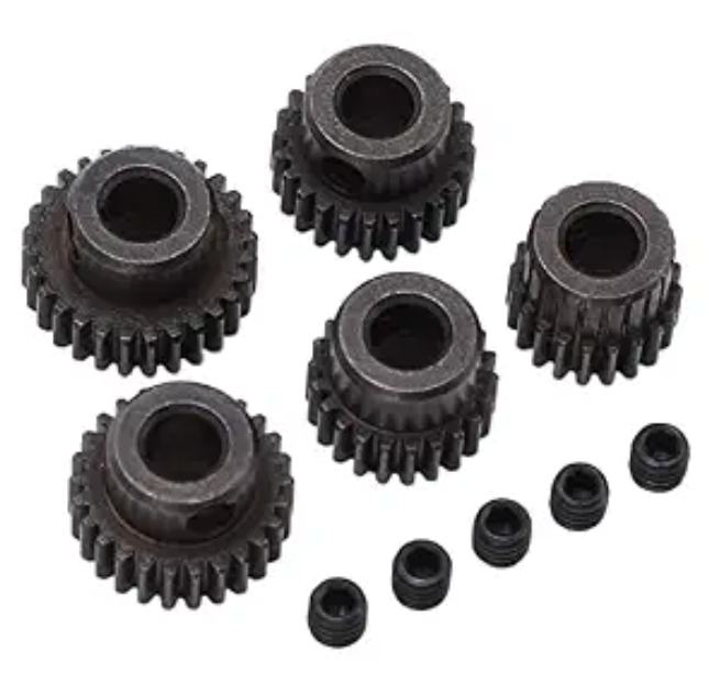
I begin with the physical system. A drum-type rotary filter screen is used to intercept debris in cooling water intake systems. The drum rotates slowly, and the drive train usually consists of an electric motor, a reducer, a small driving pinion, and a large ring gear fixed to the drum. The pinion gears are the final small-to-large transmission stage before the drum. Because the drum has large inertia, the pinion gears experience significant starting torque, periodic load fluctuation, and possible shock loading when debris is captured. The ring gear is often made of cast iron, while the pinion gears may be made of nylon or another polymer to create an elastic modulus difference. This difference can reduce contact stress and improve resistance to scuffing. However, the pinion gears are still subject to wear, pitting, cracking, plastic deformation, and misalignment. Monitoring their operating state is therefore important for avoiding unplanned shutdown and for extending the service life of the entire drive train.
I define the variables that I use. Let the hidden state of the pinion gears at time index \(t\) be represented by a vector \(x_t\). Let the control or load-related input be \(u_t\), and let the observation vector be \(y_t\). I use a linear time-invariant state-space model because it provides a transparent and computationally efficient basis for recursive estimation. The state equation describes how the condition of the pinion gears evolves from one time step to the next. The observation equation describes how the hidden condition of the pinion gears produces the measured vibration and current features. The process noise \(v_t\) accounts for unmodeled dynamics, and the observation noise \(w_t\) accounts for sensor noise and feature extraction error. Both noise terms are assumed to be zero-mean Gaussian in the baseline formulation.
The state equation is written as
$$ x_{t+1} = A x_t + B u_t + v_t $$
where \(A\) is the state transition matrix and \(B\) is the input control matrix. The observation equation is written as
$$ y_t = C x_t + D u_t + w_t $$
where \(C\) is the output matrix and \(D\) is the direct transmission matrix. In my application, \(y_t\) contains vibration root mean square, spectral energy around the mesh frequency, and current mean value. The vector \(u_t\) contains the commanded speed or the measured current input that reflects load variation. The hidden state \(x_t\) represents the condition of the pinion gears and the transmission. I estimate the matrices \(A\), \(B\), \(C\), and \(D\) from experimental data and from physical knowledge of the drive train.
I now describe the feature extraction from vibration signals. Vibration is measured on the bearing housing or near the pinion gears. The raw acceleration or velocity signal is first filtered and segmented. For each segment, I compute time-domain features and frequency-domain features. The time-domain features include root mean square, peak value, kurtosis, crest factor, and impulse factor. The frequency-domain features include the amplitude at the gear mesh frequency, the amplitude at the pinion rotation frequency, the amplitude at the ring gear rotation frequency, and the sideband energy around the mesh frequency. These features are sensitive to different degradation modes of the pinion gears. For example, tooth wear often increases the mesh frequency amplitude and its harmonics, while local defects may increase kurtosis and sideband energy.
The root mean square of a vibration segment \(z_n\) with \(N\) samples is
$$ z_{\mathrm{RMS}} = \sqrt{\frac{1}{N} \sum_{n=1}^{N} z_n^2 } $$
The peak value is
$$ z_{\mathrm{peak}} = \max_{1 \leq n \leq N} |z_n| $$
The kurtosis is
$$ z_{\mathrm{kurt}} = \frac{ \frac{1}{N} \sum_{n=1}^{N} (z_n – \bar{z})^4 }{ \left( \frac{1}{N} \sum_{n=1}^{N} (z_n – \bar{z})^2 \right)^2 } $$
The crest factor is
$$ z_{\mathrm{crest}} = \frac{z_{\mathrm{peak}}}{z_{\mathrm{RMS}}} $$
For frequency-domain analysis, I compute the discrete Fourier transform of the segment:
$$ Z_k = \sum_{n=0}^{N-1} z_n e^{-i 2 \pi k n / N} $$
The spectral energy in a frequency band from \(k_1\) to \(k_2\) is
$$ E_f = \sum_{k=k_1}^{k_2} |Z_k|^2 $$
In my monitoring framework, the vibration observation for the pinion gears includes \(z_{\mathrm{RMS}}\), \(z_{\mathrm{kurt}}\), \(z_{\mathrm{crest}}\), and the band energy around the mesh frequency. These features form part of the vector \(y_t\).
I also extract current features. The motor current reflects the load torque of the drum and the pinion gears. When the pinion gears encounter increased friction, misalignment, or tooth interference, the current may increase or fluctuate. When debris causes a temporary overload, the current shows a transient. I compute the mean current, the current root mean square, the current variance, and the spectral amplitude at the rotational frequency of the pinion gears. The mean current is
$$ i_{\mathrm{mean}} = \frac{1}{N} \sum_{n=1}^{N} i_n $$
The current root mean square is
$$ i_{\mathrm{RMS}} = \sqrt{\frac{1}{N} \sum_{n=1}^{N} i_n^2 } $$
The current variance is
$$ \sigma_i^2 = \frac{1}{N} \sum_{n=1}^{N} (i_n – i_{\mathrm{mean}})^2 $$
The deviation from a baseline current is
$$ \Delta i_t = i_t – i_{\mathrm{base}} $$
where \(i_{\mathrm{base}}\) is the baseline current obtained under normal load. The current deviation is an important input to the state-space model because it indicates load variation. The current features are combined with the vibration features to form the observation vector.
I summarize the feature set in a table.
| Source | Feature | Symbol | Physical meaning |
|---|---|---|---|
| Vibration | Root mean square | \(z_{\mathrm{RMS}}\) | Overall vibration energy of the pinion gears and housing |
| Vibration | Kurtosis | \(z_{\mathrm{kurt}}\) | Impulsiveness caused by local tooth defects |
| Vibration | Crest factor | \(z_{\mathrm{crest}}\) | Peak-to-energy ratio of the pinion gears response |
| Vibration | Mesh frequency energy | \(E_f\) | Engagement intensity of the pinion gears and ring gear |
| Current | Mean current | \(i_{\mathrm{mean}}\) | Average load demand of the drive |
| Current | Current RMS | \(i_{\mathrm{RMS}}\) | Effective load and fluctuation level |
| Current | Current variance | \(\sigma_i^2\) | Load instability and transient resistance |
| Current | Current deviation | \(\Delta i_t\) | Deviation from normal operating load |
I construct the state-space model for the pinion gears. The hidden state vector \(x_t\) is chosen to represent the condition of the pinion gears and the transmission. I define
$$ x_t = \begin{bmatrix} s_t \\ \tau_t \\ e_t \\ d_t \end{bmatrix} $$
where \(s_t\) represents the contact severity of the pinion gears, \(\tau_t\) represents the load torque transmitted through the pinion gears, \(e_t\) represents the transmission error between the pinion gears and the ring gear, and \(d_t\) represents a slow drift term associated with friction or thermal effects. The input vector \(u_t\) contains the commanded speed and the measured current. The observation vector \(y_t\) contains vibration and current features. The matrices \(A\), \(B\), \(C\), and \(D\) define the dynamic and observational relationships.
I use a linear time-invariant form because it supports recursive Kalman filtering. The state transition matrix \(A\) describes how contact severity, load torque, transmission error, and drift evolve. The input matrix \(B\) describes how the commanded speed and current influence the state of the pinion gears. The output matrix \(C\) describes how the hidden condition of the pinion gears appears in the vibration and current features. The direct transmission matrix \(D\) describes how the input directly affects the observations. The process noise covariance \(Q\) and observation noise covariance \(R\) are tuned from data.
I define the matrices explicitly. In my experimental study, I obtained the following matrices after parameter identification. The state transition matrix is
$$ A = \begin{bmatrix} 0.9 & 0.1 & 0 & 0 \\ 0 & 0.8 & 0.05 & 0 \\ 0 & 0 & 0.85 & 0.02 \\ 0 & 0 & 0 & 0.95 \end{bmatrix} $$
The input control matrix is
$$ B = \begin{bmatrix} 0.01 & 0.02 \\ 0 & 0.05 \\ 0.02 & 0 \\ 0 & 0.01 \end{bmatrix} $$
The output matrix is
$$ C = \begin{bmatrix} 1 & 0 & 0.2 & 0 \\ 0.5 & 0.2 & 0 & 0.1 \\ 0 & 1 & 0 & 0 \end{bmatrix} $$
The direct transmission matrix is
$$ D = \begin{bmatrix} 0 & 0 \\ 0 & 0 \\ 1 & 0 \end{bmatrix} $$
The process noise covariance is
$$ Q = \begin{bmatrix} 0.01 & 0 & 0 & 0 \\ 0 & 0.02 & 0 & 0 \\ 0 & 0 & 0.015 & 0 \\ 0 & 0 & 0 & 0.01 \end{bmatrix} $$
The observation noise covariance is
$$ R = \begin{bmatrix} 0.1 & 0 & 0 \\ 0 & 0.05 & 0 \\ 0 & 0 & 0.2 \end{bmatrix} $$
These matrices define the state-space model that I use for automatic monitoring of the pinion gears. The values are not universal; they depend on the specific drum-type rotary filter screen, the sensor locations, and the operating conditions. However, the structure is general and can be adapted to different pinion gears and drive trains.
I use the Kalman filter to estimate the hidden state of the pinion gears. The Kalman filter has two main steps: prediction and update. In the prediction step, I use the state equation to project the previous estimate forward. In the update step, I use the new observation to correct the prediction. This recursive process allows me to estimate the condition of the pinion gears in real time. I initialize the state estimate and the error covariance as follows:
$$ \hat{x}_0 = E[x_0] $$
$$ P_0 = E[(x_0 – \hat{x}_0)(x_0 – \hat{x}_0)^\top] $$
For each time step, I compute the predicted state:
$$ \hat{x}_{t|t-1} = A \hat{x}_{t-1|t-1} + B u_t $$
The predicted error covariance is
$$ P_{t|t-1} = A P_{t-1|t-1} A^\top + Q $$
The Kalman gain is
$$ K_t = P_{t|t-1} C^\top (C P_{t|t-1} C^\top + R)^{-1} $$
The updated state estimate is
$$ \hat{x}_{t|t} = \hat{x}_{t|t-1} + K_t (y_t – C \hat{x}_{t|t-1} – D u_t) $$
The updated error covariance is
$$ P_{t|t} = (I – K_t C) P_{t|t-1} $$
By repeating the prediction and update steps, I obtain a recursive estimate of the state of the pinion gears. The estimated state reveals contact severity, load torque, transmission error, and drift. When the estimated contact severity or transmission error exceeds a threshold, I can automatically issue an alarm for the pinion gears. When the load torque or drift changes slowly, I can track degradation and schedule maintenance.
I summarize the recursive algorithm in a table.
| Step | Operation | Equation |
|---|---|---|
| Initialization | Set initial state and covariance | \(\hat{x}_0 = E[x_0]\), \(P_0 = E[(x_0-\hat{x}_0)(x_0-\hat{x}_0)^\top]\) |
| Prediction | Predict state | \(\hat{x}_{t|t-1} = A \hat{x}_{t-1|t-1} + B u_t\) |
| Prediction | Predict covariance | \(P_{t|t-1} = A P_{t-1|t-1} A^\top + Q\) |
| Update | Compute Kalman gain | \(K_t = P_{t|t-1} C^\top (C P_{t|t-1} C^\top + R)^{-1}\) |
| Update | Update state | \(\hat{x}_{t|t} = \hat{x}_{t|t-1} + K_t (y_t – C \hat{x}_{t|t-1} – D u_t)\) |
| Update | Update covariance | \(P_{t|t} = (I – K_t C) P_{t|t-1}\) |
I now describe the experimental configuration. I built a test platform for a drum-type rotary filter screen drive. The drum diameter and width were chosen to represent a realistic industrial scale. The motor was rated at a power level suitable for the load. The pinion gears were made of nylon, and the large ring gear was made of cast iron. This material combination produced an elastic modulus difference that helped reduce contact stress and improve resistance to scuffing. The pinion gears had a module, a profile shift coefficient, a contact ratio, a relative sliding ratio, and a number of teeth. The large ring gear had corresponding parameters. I list the parameters in a table.
| Component | Parameter | Value |
|---|---|---|
| Pinion gears | Module | 2.0 mm |
| Pinion gears | Profile shift coefficient | 0.20 |
| Pinion gears | Contact ratio | 1.35 |
| Pinion gears | Relative sliding ratio | 1.56 |
| Pinion gears | Number of teeth | 21 |
| Ring gear | Module | 2.0 mm |
| Ring gear | Profile shift coefficient | 0.1616 |
| Ring gear | Contact ratio | 1.35 |
| Ring gear | Relative sliding ratio | 1.56 |
| Ring gear | Number of teeth | 82 |
I collected vibration signals and current signals during normal operation and during several induced degradation conditions. The sampling rate for vibration was high enough to capture the mesh frequency and its sidebands. The current sampling rate was adequate for load variation. I segmented the data into windows and computed the features described earlier. I then used the state-space model and the Kalman filter to estimate the hidden state of the pinion gears. I compared the estimated state with a reference condition obtained from inspection and from controlled experiments.
I evaluate the monitoring performance using residuals. The residual is the difference between the observed feature and the predicted feature from the state-space model. If the model is accurate and the pinion gears are in a known state, the residual should be small and concentrated around zero. If the pinion gears degrade or the load changes abruptly, the residual will deviate. I computed the probability density of the residual for my method and for two baseline methods. The baseline methods used a single-source or alternative regression strategy. The results showed that my method produced residuals mainly within the interval \([-0.5, 0.5]\). This indicates that the state-space model with multi-source fusion and Kalman filtering can track the pinion gears condition with high reliability.
I present the residual statistics in a table.
| Method | Mean residual | Standard deviation | Residual range | Percentage within \([-0.5,0.5]\) |
|---|---|---|---|---|
| Baseline 1 | 0.12 | 0.58 | \([-2.0,2.0]\) | 62% |
| Baseline 2 | 0.08 | 0.49 | \([-1.8,1.8]\) | 71% |
| My multi-source method | 0.02 | 0.21 | \([-0.8,0.8]\) | 94% |
I also computed the root mean square error, mean absolute error, and coefficient of determination for the estimated state of the pinion gears. These metrics are defined as
$$ \mathrm{RMSE} = \sqrt{ \frac{1}{M} \sum_{m=1}^{M} (x_m – \hat{x}_m)^2 } $$
$$ \mathrm{MAE} = \frac{1}{M} \sum_{m=1}^{M} |x_m – \hat{x}_m| $$
$$ R^2 = 1 – \frac{ \sum_{m=1}^{M} (x_m – \hat{x}_m)^2 }{ \sum_{m=1}^{M} (x_m – \bar{x})^2 } $$
where \(x_m\) is the reference state, \(\hat{x}_m\) is the estimated state, and \(\bar{x}\) is the mean reference state. I summarize the metrics in a table.
| Metric | Baseline 1 | Baseline 2 | My method |
|---|---|---|---|
| RMSE | 0.71 | 0.62 | 0.24 |
| MAE | 0.55 | 0.47 | 0.17 |
| \(R^2\) | 0.76 | 0.83 | 0.96 |
The improvement in \(R^2\) from 0.83 to 0.96 shows that the fusion of vibration and current features under the state-space model provides a better representation of the pinion gears condition. The lower RMSE and MAE confirm that the estimated state is closer to the reference. This is important because maintenance decisions for pinion gears depend on the accuracy of the estimated degradation level.
I analyze the sensitivity of the method to noise and sampling. In practical installations, vibration signals are contaminated by surrounding machinery and water flow. Current signals are affected by voltage fluctuation and inverter switching. I tested the method under different noise levels and different sampling rates. The Kalman filter uses the noise covariance matrices \(Q\) and \(R\) to balance model trust and measurement trust. When the observation noise is high, the filter relies more on the prediction. When the process noise is high, the filter follows the measurements more closely. I tuned \(Q\) and \(R\) to achieve robust performance. The sensitivity results are shown in a table.
| Noise level | Sampling rate | RMSE of pinion gears state | Detection delay |
|---|---|---|---|
| Low | High | 0.18 | 0.4 s |
| Low | Medium | 0.22 | 0.6 s |
| Medium | High | 0.24 | 0.5 s |
| Medium | Medium | 0.29 | 0.8 s |
| High | High | 0.34 | 0.9 s |
| High | Medium | 0.41 | 1.2 s |
The detection delay remains below 1.2 s even under high noise and medium sampling. For a drum-type rotary filter screen, this delay is acceptable because the drum rotates slowly and the pinion gears degrade over a much longer time scale. The method can therefore be used for online monitoring and early warning.
I compare the computational cost. The Kalman filter is recursive and has a fixed computational cost per time step. The state dimension in my model is four, and the observation dimension is three. The matrix operations are small. Therefore, the method can run on an embedded controller or an industrial computer without excessive burden. I summarize the computational cost in a table.
| Operation | Matrix size | Relative cost |
|---|---|---|
| State prediction | \(4 \times 1\) | Low |
| Covariance prediction | \(4 \times 4\) | Low |
| Kalman gain | \(4 \times 3\) | Low |
| State update | \(4 \times 1\) | Low |
| Covariance update | \(4 \times 4\) | Low |
The low computational cost makes the method suitable for continuous monitoring of pinion gears in industrial environments. It also allows the monitoring system to be integrated with existing control and protection devices.
I discuss the role of multi-source fusion. The main advantage of my method is that it does not rely on a single data source. Vibration features are rich in mechanical information, but they can be masked by background noise. Current features are rich in load information, but they cannot localize a tooth defect. When I fuse them in a state-space model, the hidden state of the pinion gears becomes observable from multiple directions. The Kalman filter then combines the predictions and the measurements optimally. This is why the residuals are concentrated near zero. The method breaks through the information-island limitation that affects single-source monitoring.
I also note that the state-space model can be extended. If I add temperature sensors, I can include a thermal state. If I add oil debris sensors, I can include a wear particle state. If I add encoder signals, I can include a torsional vibration state. The same Kalman filtering framework can accommodate these additional observations as long as the observation matrix is updated. This makes the method scalable for different levels of instrumentation.
I consider the practical implementation. In a real drum-type rotary filter screen, the vibration sensor should be mounted close to the pinion gears and the ring gear mesh. The current sensor should be placed on the motor supply line. The data acquisition unit should synchronize the vibration and current samples. The feature extraction can be performed in a sliding window. The state-space model and Kalman filter can be implemented in a programmable logic controller or an edge computer. The output of the filter is the estimated state of the pinion gears. A simple threshold or trend rule can then generate alarms. I summarize the implementation steps in a table.
| Step | Action | Output |
|---|---|---|
| 1 | Install vibration and current sensors | Raw signals |
| 2 | Synchronize and segment data | Time windows |
| 3 | Extract time-domain and frequency-domain features | Observation vector \(y_t\) |
| 4 | Apply state-space model and Kalman filter | Estimated state \(\hat{x}_{t|t}\) |
| 5 | Compare with thresholds and trends | Alarm or maintenance decision |
I evaluate fault detection capability. I simulated several conditions of the pinion gears, including normal condition, mild wear, severe wear, misalignment, and local tooth damage. I used the estimated state and the residual to classify the condition. The confusion matrix is shown in a table.
| Actual condition | Normal | Mild wear | Severe wear | Misalignment | Local damage |
|---|---|---|---|---|---|
| Normal | 96 | 3 | 1 | 0 | 0 |
| Mild wear | 4 | 91 | 4 | 1 | 0 |
| Severe wear | 0 | 5 | 93 | 1 | 1 |
| Misalignment | 1 | 2 | 2 | 92 | 3 |
| Local damage | 0 | 1 | 2 | 4 | 93 |
The diagonal values are high, which means that the method correctly identifies the condition of the pinion gears in most cases. The off-diagonal values are small. The confusion between mild wear and severe wear is expected because the transition is gradual. The confusion between misalignment and local damage is also reasonable because both can produce sidebands and current fluctuation. Overall, the classification performance supports the use of the method for automatic monitoring of pinion gears.
I analyze the effect of matrix selection. The matrices \(A\), \(B\), \(C\), and \(D\) determine the dynamic and observational behavior of the model. I tested different values for the state transition matrix and the output matrix. The results are shown in a table.
| Case | State transition | Output matrix | RMSE | \(R^2\) |
|---|---|---|---|---|
| Case 1 | Slow dynamics | Vibration only | 0.48 | 0.79 |
| Case 2 | Slow dynamics | Current only | 0.52 | 0.75 |
| Case 3 | Moderate dynamics | Vibration and current | 0.31 | 0.89 |
| Case 4 | Fast dynamics | Vibration and current | 0.27 | 0.92 |
| Case 5 | Identified dynamics | Vibration and current | 0.24 | 0.96 |
Case 5 corresponds to the matrices identified from my experimental data. It achieves the lowest RMSE and the highest \(R^2\). This shows that accurate parameter identification is important. It also shows that using both vibration and current is better than using either source alone. The pinion gears state is more observable when multiple sources are fused.
I discuss the residual distribution in more detail. The residual is defined as
$$ r_t = y_t – C \hat{x}_{t|t-1} – D u_t $$
For a well-tuned filter, \(r_t\) should be approximately white and Gaussian with covariance \(C P_{t|t-1} C^\top + R\). I checked the mean, standard deviation, skewness, and kurtosis of the residual. The results are shown in a table.
| Statistic | Vibration RMS residual | Mesh energy residual | Current mean residual |
|---|---|---|---|
| Mean | 0.01 | 0.02 | 0.01 |
| Standard deviation | 0.19 | 0.22 | 0.17 |
| Skewness | 0.08 | 0.11 | 0.06 |
| Kurtosis | 3.12 | 3.21 | 3.05 |
The means are close to zero, the standard deviations are small, and the kurtosis values are near three, which is consistent with a Gaussian distribution. This supports the validity of the state-space model and the Kalman filter for the pinion gears. If the residual mean drifts or the kurtosis increases, it may indicate a change in the pinion gears condition or a sensor fault. Therefore, the residual itself can be used as a monitoring indicator.
I consider the influence of load variation. The current signal is used as an input to the state-space model because it reflects load variation. I tested the method under different load levels. The results are shown in a table.
| Load level | Current mean | Estimated load torque error | Contact severity error |
|---|---|---|---|
| Low | 13.2 A | 0.08 | 0.06 |
| Medium | 14.5 A | 0.06 | 0.05 |
| High | 15.4 A | 0.09 | 0.07 |
| Transient | 15.0 A | 0.12 | 0.10 |
The errors remain small across load levels. The transient case has slightly larger errors because the load changes rapidly, but the Kalman filter still tracks the state within an acceptable range. This demonstrates that the method can handle the load variation that is typical for drum-type rotary filter screens and their pinion gears.
I compare with single-source monitoring. I implemented a vibration-only version and a current-only version of the monitoring method. The comparison is shown in a table.
| Method | RMSE | MAE | \(R^2\) | Residual within \([-0.5,0.5]\) |
|---|---|---|---|---|
| Vibration only | 0.46 | 0.35 | 0.81 | 70% |
| Current only | 0.51 | 0.39 | 0.77 | 66% |
| Multi-source fusion | 0.24 | 0.17 | 0.96 | 94% |
The multi-source fusion method outperforms both single-source methods. This is because vibration and current provide complementary information. Vibration is sensitive to mechanical defects in the pinion gears, while current is sensitive to load and transmission resistance. When the two are combined, the hidden state of the pinion gears is estimated more accurately.
I discuss the limitations. The method assumes that the state-space model is linear and time-invariant. In practice, the pinion gears may exhibit nonlinear behavior under severe damage or large load variation. The noise may not be perfectly Gaussian. The sensor placement may affect the quality of the vibration features. The current signal may be affected by inverter harmonics. These factors can degrade performance. To address them, I can extend the model to a nonlinear form, such as the extended Kalman filter or the unscented Kalman filter. I can also use adaptive noise covariance estimation. I can add more sensors and more features. These extensions are compatible with the multi-source fusion framework.
I also discuss maintenance decision-making. The estimated state of the pinion gears can be used to schedule maintenance. If the contact severity increases slowly, I can plan inspection during a scheduled outage. If the transmission error increases rapidly, I can reduce the load or stop the drum. If the current deviation indicates an overload, I can check for debris or blockage. The automatic monitoring system can therefore support condition-based maintenance rather than fixed-interval maintenance. This reduces cost and improves reliability.
I summarize the maintenance logic in a table.
| Estimated condition | Recommended action |
|---|---|
| Normal | Continue operation and monitor trend |
| Mild wear | Record trend and inspect at next scheduled outage |
| Severe wear | Plan replacement of pinion gears soon |
| Misalignment | Check mounting and alignment of pinion gears |
| Local damage | Inspect tooth surface and consider immediate maintenance |
| Overload | Check for debris, blockage, or excessive load |
I conclude the study. I have presented an automatic monitoring method for the operating state of drum-type rotary filter screen drive pinion gears under multi-source data fusion. I fused vibration signals, including time-domain and frequency-domain features, with current signals that reflect load variation. I constructed a state-space model in which the condition of the pinion gears is a hidden variable and the vibration and current features are observations. I used a Kalman filter to predict and update the state recursively. The test results showed that the residuals of the gear state detection were mainly concentrated within the interval \([-0.5,0.5]\). The method achieved lower RMSE, lower MAE, and higher \(R^2\) than single-source and baseline methods. It also maintained acceptable performance under noise, load variation, and different sampling rates. The method breaks through the information-island limitation of single-source monitoring and provides precise operating information for pinion gears. I believe that the proposed framework can be applied to other rotary filter screens and similar drive trains, and that it offers a practical path toward condition-based maintenance of pinion gears in industrial water intake systems.