
As a researcher focusing on nonlinear dynamics and intelligent control, I have long been fascinated by the complex behavior of straight bevel gear transmission systems. These systems are ubiquitous in locomotive traction mechanisms, where they must endure high torque, frequent start-stop cycles, and severe load fluctuations. The straight bevel gear is a critical component that transmits motion between intersecting axes, often at a 90-degree angle. Its advantages include high load capacity, smooth transmission, large gear ratio, and structural simplicity. However, the presence of nonlinear factors such as time-varying mesh stiffness, backlash, transmission error, and damping can drive the straight bevel gear system into chaotic motion, leading to excessive vibration, noise, and premature failure. In this article, I present my comprehensive investigation into the nonlinear dynamics of a straight bevel gear transmission system and propose an intelligent chaos control strategy based on a fuzzy neural network (FNN) optimized by an improved particle swarm optimization (IPSO) algorithm. My goal is to steer the chaotic, quasi-periodic, or multi-periodic motions of the straight bevel gear system onto stable periodic orbits, thereby enhancing operational reliability and extending equipment life.
Throughout my research, I have established a seven-degree-of-freedom (7-DOF) dynamic model of a straight bevel gear pair, analyzed its bifurcation characteristics under various parameters, designed a five-layer FNN controller, and developed an IPSO algorithm with chaotic initialization, adaptive learning factors, adaptive inertia weight, and a dynamic centroid migration-based Lévy flight mechanism. I validated the proposed control scheme through extensive numerical simulations. The results demonstrate that my IPSO-FNN controller can rapidly and effectively suppress chaos in the straight bevel gear system, achieving period-1, period-2, period-4, and other targeted periodic motions. This work provides a theoretical reference for avoiding chaotic vibrations in straight bevel gear transmissions.
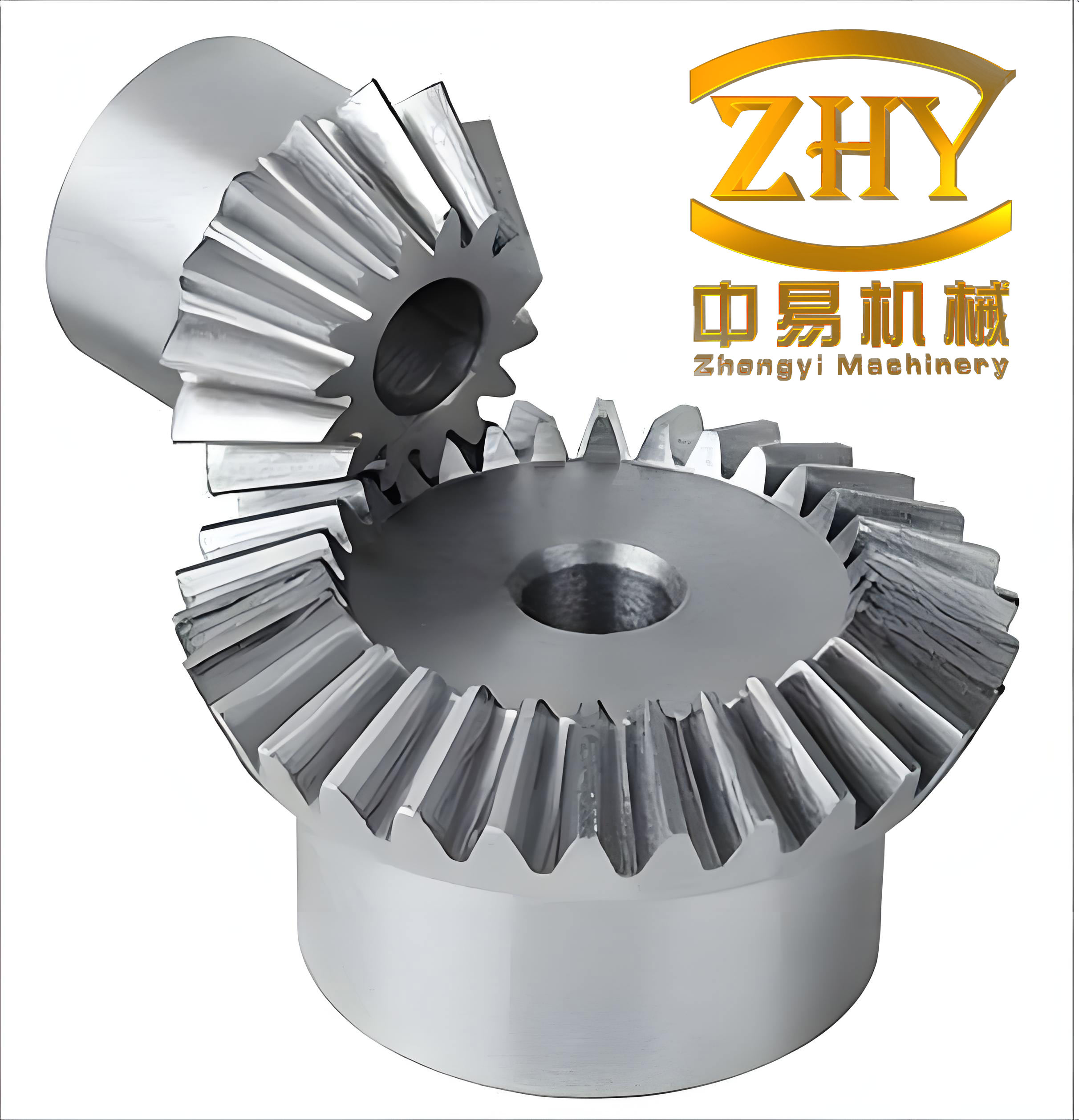
To give readers a clear view of a typical straight bevel gear, I include the following image. It shows the intricate geometry of the gear teeth and the overall structure that I modeled.
1. Nonlinear Dynamic Modeling of the Straight Bevel Gear System
I began by constructing a lumped-mass model of a straight bevel gear pair. The system consists of a driving gear and a driven gear, each with translational and rotational degrees of freedom. I considered time-varying mesh stiffness, comprehensive transmission error, backlash, and meshing damping. The basic geometric parameters of the straight bevel gear pair used in my study are listed in Table 1.
| Parameter | Symbol | Driving gear | Driven gear |
|---|---|---|---|
| Number of teeth | $z_1, z_2$ | 47 | 53 |
| Module (mm) | $m$ | 2 | 2 |
| Pressure angle at pitch cone (°) | $\alpha_n$ | 20 | 20 |
| Pitch cone angle (°) | $\delta_1, \delta_2$ | 41.57 | 48.43 |
| Addendum coefficient | $h^*$ | 1 | 1 |
| Clearance coefficient | $c^*$ | 0.25 | 0.25 |
| Cone distance (mm) | $R$ | 70.8 | 70.8 |
| Tip angle (°) | $\theta_{a1}, \theta_{a2}$ | 2.35 | 1.95 |
| Tip cone angle (°) | $\delta_{a1}, \delta_{a2}$ | 43.92 | 50.34 |
| Root angle (°) | $\theta_{f1}, \theta_{f2}$ | 1.95 | 2.35 |
| Root cone angle (°) | $\delta_{f1}, \delta_{f2}$ | 39.62 | 46.04 |
| Gear ratio | $u$ | 1.13 | |
| Modification coefficient | $x_1, x_2$ | 0.04 | -0.04 |
| Addendum (mm) | $h_{a1}, h_{a2}$ | 2.08 | 1.92 |
| Tooth height (mm) | $h$ | 4.5 | |
| Dedendum (mm) | $h_{f1}, h_{f2}$ | 2.42 | 2.58 |
| Pitch diameter (mm) | $d_1, d_2$ | 94 | 106 |
Using Newton’s second law, I derived the equations of motion for the 7-DOF straight bevel gear system. The degrees of freedom include three translational displacements for each gear and one rotational displacement for each gear, but after eliminating the rigid-body rotation, the system reduces to seven relative coordinates. The dynamic equations are:
$$
\begin{cases}
I_1 \ddot{\theta}_1 + r_1 F_n = T_1, \\
I_2 \ddot{\theta}_2 – r_2 F_n = -T_2, \\
m_1 \ddot{y}_1 + c_{y1} \dot{y}_1 + k_{y1} y_1 = F_y, \\
m_2 \ddot{y}_2 + c_{y2} \dot{y}_2 + k_{y2} y_2 = -F_y, \\
m_1 \ddot{z}_1 + c_{z1} \dot{z}_1 + k_{z1} z_1 = F_z, \\
m_2 \ddot{z}_2 + c_{z2} \dot{z}_2 + k_{z2} z_2 = -F_z, \\
m_1 \ddot{x}_1 + c_{x1} \dot{x}_1 + k_{x1} x_1 = F_x, \\
m_2 \ddot{x}_2 + c_{x2} \dot{x}_2 + k_{x2} x_2 = -F_x,
\end{cases}
$$
where $\theta_i$ are the torsional displacements, $T_i$ are the torques, $m_i$ are the masses, $I_i$ are the moments of inertia, $c_{ij}$ and $k_{ij}$ are the support damping and stiffness, and $F_n$, $F_x$, $F_y$, $F_z$ are the dynamic mesh force components. The relative torsional displacement along the line of action is defined as:
$$
\lambda = (x_1 – x_2)\alpha_1 + (y_1 – y_2)\alpha_2 + (z_1 – z_2)\alpha_3 – (r_1\theta_1 – r_2\theta_2) – e(t),
$$
where $\alpha_1 = \cos\delta_1 \sin\alpha_n$, $\alpha_2 = \cos\delta_1 \cos\alpha_n$, $\alpha_3 = \cos\alpha_n$, and $e(t)$ is the comprehensive transmission error. The dynamic mesh force is:
$$
F_n = k_h(t) f(\lambda, b) + c_h \dot{\lambda},
$$
with the backlash function:
$$
f(\lambda, b) =
\begin{cases}
\lambda – b, & \lambda > b, \\
0, & |\lambda| \le b, \\
\lambda + b, & \lambda < -b.
\end{cases}
$$
To simplify the analysis, I nondimensionalized the equations. Let $\tau = \omega_n t$, $x_j = X_j/b_h$, $y_j = Y_j/b_h$, $z_j = Z_j/b_h$, and introduce the dimensionless parameters: $\Omega = \omega_h / \omega_n$, $\xi_{ij} = c_{ij}/(2m_j\omega_n)$, $\xi_{hj} = c_h/(2\omega_n m_j)$, $\xi_h = c_h/(2m_e\omega_n)$, $f_{pm} = F_{pm}/(\omega_n^2 b_h m_e)$, $f_e = e_l/b_h$, $a = k_{kl}/k_m$, and $k_h(\tau) = 1 + a\cos(\Omega\tau)$. The dimensionless equations of motion become a set of 14 first-order state equations:
$$
\begin{aligned}
\dot{x}_1 &= x_2, \\
\dot{x}_2 &= -2\xi_{x1} x_2 – k_{x1} x_1 + k_{h1} f(x_{13}, b) + c_4 x_{14}, \\
\dot{x}_3 &= x_4, \\
\dot{x}_4 &= -2\xi_{y1} x_4 – k_{y1} x_3 + k_{h1} f(x_{13}, b) + c_5 x_{14}, \\
&\vdots \\
\dot{x}_{13} &= x_{14}, \\
\dot{x}_{14} &= -c_1 x_2 – c_2 x_4 – c_3 x_6 – c_1 x_8 – c_2 x_{10} – c_3 x_{12} \\
&\quad – 2\xi_h x_{14} – k_h f(x_{13}, b) + f_{pm} + f_e \cos(\Omega\tau),
\end{aligned}
$$
where $x_{13} = \lambda/b_h$ and the coefficients $c_i$ depend on the cone angles and pressure angle. I solved these equations numerically using the fourth-fifth order Runge-Kutta method.
2. Bifurcation Analysis of the Straight Bevel Gear System
To understand the chaotic behavior of the straight bevel gear system, I performed extensive bifurcation analysis. I varied four key parameters: the time-varying mesh stiffness coefficient $a$, the comprehensive transmission error coefficient $f_e$, the load coefficient $f_{pm}$, and the mesh frequency ratio $\Omega$. I used bifurcation diagrams, phase portraits, and Poincaré sections to identify periodic, quasi-periodic, and chaotic regions. Table 2 summarizes the observed dynamical behaviors as each parameter varies.
| Parameter | Range | Observed behavior |
|---|---|---|
| $a$ (mesh stiffness coefficient) | 0.1 – 0.35 | Chaotic motion |
| 0.35 – 0.40 | Period-3 motion | |
| 0.40 – 0.43 | Period-6 and period-12 via period doubling | |
| 0.43 – 1.00 | Quasi-periodic then chaotic at higher values | |
| $f_e$ (transmission error coefficient) | 0 – 0.1048 | Period-1 |
| 0.1048 – 0.149 | Period-2, period-4, period-8 | |
| 0.149 – 0.2315 | Chaotic with periodic windows | |
| 0.2315 – 0.378 | Period-3, period-6, period-12 | |
| 0.378 – 2.00 | Alternating chaos, period-4, period-2, period-1 | |
| $f_{pm}$ (load coefficient) | 0 – 0.00151 | Period-1 |
| 0.00151 – 0.00248 | Period-2 | |
| 0.00248 – 0.04 | Chaotic | |
| 0.04 – 1.00 | Quasi-periodic, period-9, period-6, period-4, period-2, period-1 | |
| $\Omega$ (mesh frequency ratio) | 0.50 – 0.83 | Period-1, period-2, period-4 |
| 0.83 – 1.03 | Period-8, multi-periodic, chaotic | |
| 1.03 – 1.10 | Period-3, period-6 | |
| 1.10 – 1.25 | Chaotic with periodic windows | |
| 1.25 – 2.00 | Quasi-periodic, period-4, period-2, period-1 |
For instance, when I set $a = 0.3$, the phase portrait of the straight bevel gear system showed a tangled, folded trajectory, and the Poincaré map exhibited a non-periodic set of points, confirming chaotic motion. At $a = 0.35$, the system transitioned to period-3 motion, and further increases in $a$ led to period-doubling bifurcations. When I varied $f_e$, I observed a classic route to chaos: period-1 → period-2 → period-4 → period-8 → chaos, followed by periodic windows. For the load coefficient $f_{pm}$, the straight bevel gear system exhibited rich dynamics including period-9, period-6, and period-3 motions embedded within quasi-periodic or chaotic regions. Similarly, the mesh frequency ratio $\Omega$ produced alternating chaotic and periodic bands. These findings highlight the importance of avoiding chaotic parameter regions in practical straight bevel gear design.
To quantify the chaotic regions, I computed the largest Lyapunov exponent for selected parameter values. Table 3 lists some representative cases.
| Parameter set | Largest Lyapunov exponent | Motion type |
|---|---|---|
| $a = 0.25, \Omega = 0.862$ | 0.152 | Chaotic |
| $a = 0.25, \Omega = 1.066$ | -0.021 | Period-3 |
| $a = 0.25, \Omega = 1.23$ | -0.008 | Multi-periodic |
| $a = 0.25, f_{pm} = 0.002$ | 0.134 | Chaotic |
| $a = 0.25, f_{pm} = 0.016$ | -0.015 | Quasi-periodic |
3. Design of the Fuzzy Neural Network Chaos Controller
To control the chaotic motion of the straight bevel gear system, I designed a five-layer fuzzy neural network (FNN) controller. The controller takes two inputs: the Euclidean distance between two adjacent points on the Poincaré section after the $k$-th iteration, $d(k) = \|X(k) – X(k-1)\|$, and the distance after the $(k-1)$-th iteration, $d(k-1) = \|X(k-1) – X(k-2)\|$. The output is a small perturbation $U(k)$ applied to a controllable parameter, such as the mesh frequency ratio $\Omega$ or the load coefficient $f_{pm}$. The structure of my FNN controller is shown in Table 4.
| Layer | Function | Number of nodes | Equation |
|---|---|---|---|
| Input layer | Receives $d(k)$ and $d(k-1)$ | 2 | $D(k) = [d(k), d(k-1)]^T$ |
| Fuzzification layer | Gaussian membership functions | 2 × 5 = 10 | $\mu_{im} = \exp\left(-\frac{\|D_i – C_{im}\|^2}{b_{im}^2}\right)$ |
| Rule layer | Fuzzy inference (product) | 5 | $a_i = \mu_{1i} \mu_{2i}$ |
| Defuzzification layer | Normalization | 5 | $\bar{a}_i = a_i / \sum_{j=1}^5 a_j$ |
| Output layer | Weighted sum | 1 | $U(k) = \sum_{i=1}^5 \bar{a}_i w_i$ |
The membership functions are Gaussian, with centers $C_{im}$ and widths $b_{im}$. The weights $w_i$ connect the defuzzification layer to the output layer. The controller output is constrained by $|U(k)| \le u_{max}$, where $u_{max}$ is the maximum allowable perturbation. The fitness function for optimizing the controller parameters is defined as:
$$
F_i = \sum_{k=1}^{L} \left( d^* – \|X(k) – X(k-1)\| \right)^2,
$$
where $d^*$ is the desired distance between adjacent Poincaré points (which depends on the target periodic orbit) and $L$ is the length of the data sequence. I used an improved particle swarm optimization (IPSO) algorithm to find the optimal parameters $w$, $b$, and $c$ for the FNN controller.
4. Improved Particle Swarm Optimization Algorithm
The standard particle swarm optimization (PSO) algorithm often suffers from premature convergence and local optima, especially for high-dimensional problems like tuning a fuzzy neural network. To overcome these limitations, I developed an improved PSO (IPSO) algorithm with four key enhancements: (1) chaotic initialization of particle positions using a Piecewise map, (2) adaptive learning factors, (3) nonlinear adaptive inertia weight, and (4) a dynamic centroid migration-based Lévy flight mechanism. I also introduced a Bernoulli-based selection mechanism to coordinate the Lévy flight with the standard velocity update.
The Piecewise chaotic map for initialization is:
$$
p(t+1) =
\begin{cases}
\frac{p(t)}{q}, & 0 \le p(t) < q, \\
\frac{p(t)-q}{0.5-q}, & q \le p(t) < 0.5, \\
\frac{1-q-p(t)}{0.5-q}, & 0.5 \le p(t) < 1-q, \\
\frac{1-p(t)}{q}, & 1-q \le p(t) \le 1,
\end{cases}
$$
with $q = 1$ for my implementation. The adaptive learning factors are:
$$
c_1 = 2 \sin\left(\frac{\pi}{2}\left(1 – \frac{t}{T}\right)\right), \quad
c_2 = 2 \sin\left(\frac{\pi}{2}\frac{t}{T}\right),
$$
where $t$ is the current iteration and $T$ is the maximum number of iterations. The nonlinear adaptive inertia weight is:
$$
w = w_{max} – (w_{max} – w_{min}) \tan\left(0.875\left(1 – \left(\frac{t}{T}\right)^k\right)\right),
$$
with $w_{max} = 0.9$, $w_{min} = 0.1$, and $k = 0.6$. For the Lévy flight, I used:
$$
p_{is}(t+1) = b_1 p_{is}(t) + b_2 \left( p_{gbest} + 0.01 \cdot s \cdot (p_{is}(t) – p_{gbest}) \right),
$$
where $s = \mu / |\nu|^{1/\beta}$, with $\mu \sim N(0, \sigma_\mu^2)$, $\nu \sim N(0, 1)$, and $\beta = 1.5$. The parameters $b_1$ and $b_2$ change dynamically to shift the search focus from exploration to exploitation. The overall position update uses a Bernoulli selection:
$$
p_{is}(t+1) =
\begin{cases}
p_{is}(t) + v_{is}(t+1), & A < 0.5, \\
b_1 p_{is}(t) + b_2 \left( p_{gbest} + 0.01 s (p_{is}(t) – p_{gbest}) \right), & A \ge 0.5,
\end{cases}
$$
where $A$ is a random number in [0,1]. I tested the IPSO algorithm on eight benchmark functions. Table 5 compares the best results obtained by standard PSO and my IPSO.
| Function | Standard PSO | IPSO |
|---|---|---|
| Ackley | 5.0574e-04 | 8.8817e-16 |
| Alpine | 0.145318988148 | 6.0014e-141 |
| Eggholder | 7.9501e+02 | 9.5964e+02 |
| Griewank | 1.1504e-07 | 0 |
| Levy | 0.090218101524063 | 3.0395e-07 |
| Rastrigin | 8.188847064707494 | 0 |
| Schaffer | -0.995115820950763 | -1 |
| Weierstrass | 2.503866314153974 | 0 |
Clearly, IPSO outperforms standard PSO in terms of accuracy and ability to escape local optima. I then used IPSO to optimize the FNN controller parameters $w$, $b$, and $c$. The parameter ranges were $w \in [-3, 3]$, $b \in [-3, 3]$, and $c \in [-3, 3]$. The population size was $N = 150$, and the maximum number of iterations was $T = 100$.
5. Simulation Results of Chaos Control for the Straight Bevel Gear System
I applied the IPSO-FNN controller to the straight bevel gear system to control chaotic, multi-periodic, and quasi-periodic motions. I considered two controllable parameters: the mesh frequency ratio $\Omega$ and the load coefficient $f_{pm}$. The controller started to apply perturbations after 200 iterations of the system. For each case, I recorded the orbit diagram, phase portrait, Poincaré section, and perturbation magnitude.
5.1 Controlling Chaos to Period-1, Period-2, and Period-4
First, I set the initial mesh frequency ratio $\Omega = 0.862$, where the straight bevel gear system exhibited chaotic motion. The phase portrait showed a tangled trajectory, and the Poincaré section had non-periodic points. After activating the controller, the system quickly converged to a stable period-1 orbit. The perturbation magnitude remained small and became constant. The controller parameters for this case are listed in Table 6.
| $w$ | $b_{1m}, b_{2m}$ | $C_{1m}, C_{2m}$ |
|---|---|---|
| -1.7350 | -1.5721, -1.2846 | -1.6693, -1.7799 |
| -0.1285 | -1.6599, -1.3353 | -0.8814, -0.6160 |
| -1.7931 | -0.9319, -0.3782 | -0.9916, -1.2283 |
| -0.2182 | -1.2521, -0.7416 | -0.6149, -1.1715 |
| -0.3479 | -1.5100, -0.5805 | -0.1482, 0.6168 |
Next, I targeted period-2 motion. The straight bevel gear system reached the period-2 orbit after only 4 perturbations. The Poincaré section showed exactly two points. Table 7 gives the controller parameters for this case.
| $w$ | $b_{1m}, b_{2m}$ | $C_{1m}, C_{2m}$ |
|---|---|---|
| -0.0803 | -1.4886, 0.9841 | 0.1473, 0.1163 |
| 0.4621 | -0.4757, 0.0399 | 0.2704, 1.0648 |
| 0.3427 | 1.6503, -0.1176 | -0.6700, -1.2135 |
| 0.0148 | -0.8108, 0.2946 | -0.4539, -1.0073 |
| -0.5040 | 0.4740, 0.0034 | -0.1899, -0.1414 |
For period-4 control, the straight bevel gear system converged after about 10 perturbations. The Poincaré section displayed four points. Table 8 shows the optimized parameters.
| $w$ | $b_{1m}, b_{2m}$ | $C_{1m}, C_{2m}$ |
|---|---|---|
| -0.3808 | -1.9091, -2.4368 | -1.3317, -3.0000 |
| -0.8313 | -0.5714, -2.1608 | -3.0000, -2.4170 |
| -2.6842 | -1.0141, -0.2008 | -2.2337, -1.6978 |
| -1.0908 | -2.7536, -0.0543 | -1.9870, -1.5736 |
| -1.0023 | -1.4612, -1.0337 | -2.0165, -2.5512 |
5.2 Controlling Multi-Periodic Motion
I also tested the controller on multi-periodic motions. With $\Omega = 1.23$, the straight bevel gear system initially exhibited a multi-periodic state. The IPSO-FNN controller successfully steered it to period-4 in 6 perturbations. Table 9 lists the controller parameters.
| $w$ | $b_{1m}, b_{2m}$ | $C_{1m}, C_{2m}$ |
|---|---|---|
| -0.1367 | -2.1635, -2.3862 | -0.4952, -2.5571 |
| -0.1795 | -2.5761, -0.1598 | 0.4362, 2.0490 |
| -1.9758 | -2.6333, -0.3840 | 0.0898, -2.0714 |
| 0.6067 | -0.0083, -1.9657 | -2.6324, -2.2060 |
| 0.1060 | -0.3019, -0.1404 | -2.0047, -1.0362 |
With $\Omega = 1.256$, the straight bevel gear system was multi-periodic. The controller drove it to period-2 after 5 perturbations. The parameters are given in Table 10.
| $w$ | $b_{1m}, b_{2m}$ | $C_{1m}, C_{2m}$ |
|---|---|---|
| -0.0860 | -0.2337, -0.2914 | -0.3830, 0.0324 |
| 0.2936 | -0.2419, -0.2212 | -0.2916, -0.9098 |
| 0.0336 | 0.1427, -0.0342 | -0.1172, -0.2678 |
| -0.0086 | -0.1308, -0.1198 | 0.0809, 0.0434 |
| -0.0457 | -0.1515, -0.0812 | -0.1964, -0.2044 |
Similarly, when starting from the same multi-periodic state, the controller could also achieve period-1 motion. Table 11 shows the corresponding parameters.
| $w$ | $b_{1m}, b_{2m}$ | $C_{1m}, C_{2m}$ |
|---|---|---|
| 0.1520 | 0.2960, 0.0481 | 0.1774, 0.2360 |
| 0.0837 | 0.2450, 0.4161 | 0.4629, 0.1254 |
| 0.0351 | 0.3020, 0.1284 | 0.1555, 0.1165 |
| 0.2082 | 0.3115, 0.2060 | 0.1518, 0.1327 |
| 0.0770 | 0.0528, 0.5369 | 0.1729, 0.0957 |
5.3 Controlling Using the Load Coefficient as the Perturbation Parameter
To demonstrate the versatility of my approach, I also used the load coefficient $f_{pm}$ as the control parameter. With initial $f_{pm} = 0.002$, the straight bevel gear system was chaotic. The IPSO-FNN controller steered it to period-2 after 20 perturbations. Table 12 lists the parameters.
| $w$ | $b_{1m}, b_{2m}$ | $C_{1m}, C_{2m}$ |
|---|---|---|
| 0.8521 | -0.6408, 0.0869 | 0.7505, 0.5505 |
| 1.1088 | 0.0077, -0.6882 | 1.2175, 1.0331 |
| -0.2776 | -1.0447, -0.8659 | 1.2129, -1.6556 |
| 0.2193 | -0.0434, -1.0045 | 0.6876, 0.3119 |
| -0.7776 | 0.2196, -0.2264 | 0.7880, 0.2864 |
When the initial load coefficient was $f_{pm} = 0.016$, the straight bevel gear system exhibited quasi-periodic motion. The controller again achieved period-2 in only 5 perturbations. Table 13 provides the parameters.
| $w$ | $b_{1m}, b_{2m}$ | $C_{1m}, C_{2m}$ |
|---|---|---|
| -0.0860 | -0.2337, -0.2914 | -0.3830, 0.0324 |
| 0.2936 | -0.2419, -0.2212 | -0.2916, -0.9098 |
| 0.0336 | 0.1427, -0.0342 | -0.1172, -0.2678 |
| -0.0086 | -0.1308, -0.1198 | 0.0809, 0.0434 |
| -0.0457 | -0.1515, -0.0812 | -0.1964, -0.2044 |
In all cases, the perturbation magnitude remained small, and the straight bevel gear system rapidly entered a stable periodic orbit. These results confirm that my IPSO-FNN controller is effective for a wide range of chaotic and non-chaotic undesirable motions in the straight bevel gear transmission system.
6. Conclusion and Future Work
I have conducted a comprehensive study on the nonlinear dynamics and chaos control of a straight bevel gear transmission system. My main contributions are as follows:
- I established a 7-DOF dynamic model of a straight bevel gear pair, incorporating time-varying mesh stiffness, comprehensive transmission error, backlash, and damping. I derived the dimensionless state equations and solved them using the Runge-Kutta method.
- I analyzed the bifurcation characteristics of the straight bevel gear system under variations of mesh stiffness coefficient, transmission error coefficient, load coefficient, and mesh frequency ratio. I identified chaotic, quasi-periodic, and multi-periodic regions, providing guidance for avoiding undesirable vibrations.
- I designed a five-layer fuzzy neural network controller with two inputs and one output, and I proposed an improved particle swarm optimization algorithm with chaotic initialization, adaptive learning factors, adaptive inertia weight, and a dynamic centroid migration-based Lévy flight mechanism.
- I validated the IPSO algorithm on eight benchmark functions, demonstrating its superior global search capability and convergence accuracy compared to standard PSO.
- I applied the IPSO-FNN controller to the straight bevel gear system and successfully controlled chaotic, multi-periodic, and quasi-periodic motions to period-1, period-2, and period-4 orbits using either the mesh frequency ratio or the load coefficient as the control parameter.
My results show that the IPSO-FNN controller can rapidly and precisely steer the straight bevel gear system to stable periodic orbits, thereby avoiding chaotic vibrations that could compromise reliability. This intelligent control strategy offers a theoretical reference for the design and operation of straight bevel gear transmissions in locomotives and other machinery.
For future work, I plan to incorporate more nonlinear factors such as thermo-elastohydrodynamic lubrication and friction into the straight bevel gear model to improve its engineering applicability. I also intend to design a bench experiment to validate my numerical findings through vibration and torque measurements. By combining simulation and experiment, I hope to further refine the control strategy and extend it to other types of gear systems.
In summary, the straight bevel gear is a vital component in many mechanical systems, and its chaotic behavior must be controlled to ensure safe and reliable operation. My research provides a promising solution based on fuzzy neural networks and improved particle swarm optimization. I believe that this work will inspire further studies on intelligent chaos control for straight bevel gear transmission systems and other nonlinear dynamic systems.