
In this work, I investigate the nonlinear dynamic behavior of helical gears in a high-speed train gearbox and develop an intelligent control strategy to suppress chaotic vibration. I treat the helical gears as a coupled six-degree-of-freedom mechanical system, because the axial, transverse, and torsional motions of helical gears interact strongly through the normal mesh force and the helix angle. My objective is not only to identify where chaotic vibration appears in helical gears, but also to drive the system from chaotic, quasi-periodic, and multi-periodic states into prescribed periodic states by applying small perturbations to controllable parameters. I use a radial basis function neural network controller and a back-propagation neural network controller, and I optimize their parameters with an improved gravitational search algorithm. The main contribution is a complete numerical framework that connects nonlinear modeling, bifurcation analysis, controller design, optimization, and control verification for helical gears.
1. Motivation and Scope
Helical gears are widely used in train gearboxes because they transmit large torque with smoother contact than spur gears. However, the same helix angle that improves load sharing also introduces axial force components, coupling between bending, torsional, and axial motions, and additional sensitivity to manufacturing and assembly errors. When time-varying mesh stiffness, transmission error, backlash, damping, and load fluctuations act together, helical gears can exhibit period-doubling, saddle-node bifurcation, quasi-periodic motion, and chaos. Chaotic vibration in helical gears is undesirable because it can increase dynamic load, aggravate tooth surface impact, produce noise, and reduce the reliability of the entire transmission system.
I focus on the following questions. First, how do the primary nonlinear factors of helical gears influence impact state, contact loss, back-side contact, and dynamic load? Second, where do chaotic and periodic windows appear in the parameter plane? Third, can a neural network controller with a small perturbation drive helical gears to a desired periodic orbit without requiring an exact Jacobian matrix? Fourth, how can the gravitational search algorithm be improved so that controller parameters are accurate enough for chaotic helical gears? I answer these questions through numerical simulation and comparative control experiments.
2. Nonlinear Dynamic Model of Helical Gears
I model the helical gears as two rigid bodies connected by a time-varying mesh stiffness and a mesh damping element. Each gear has two transverse displacements and one rotation, so the complete system has six degrees of freedom. The symbol \(Y_i\) denotes transverse displacement in one direction, \(Z_i\) denotes transverse displacement in the perpendicular direction, and \(\theta_i\) denotes rotation. The subscript \(i=1\) denotes the driving gear, and \(i=2\) denotes the driven gear. The dynamic mesh force of the helical gears depends on the relative displacement along the normal mesh line, the backlash function, the time-varying mesh stiffness, and the mesh damping.
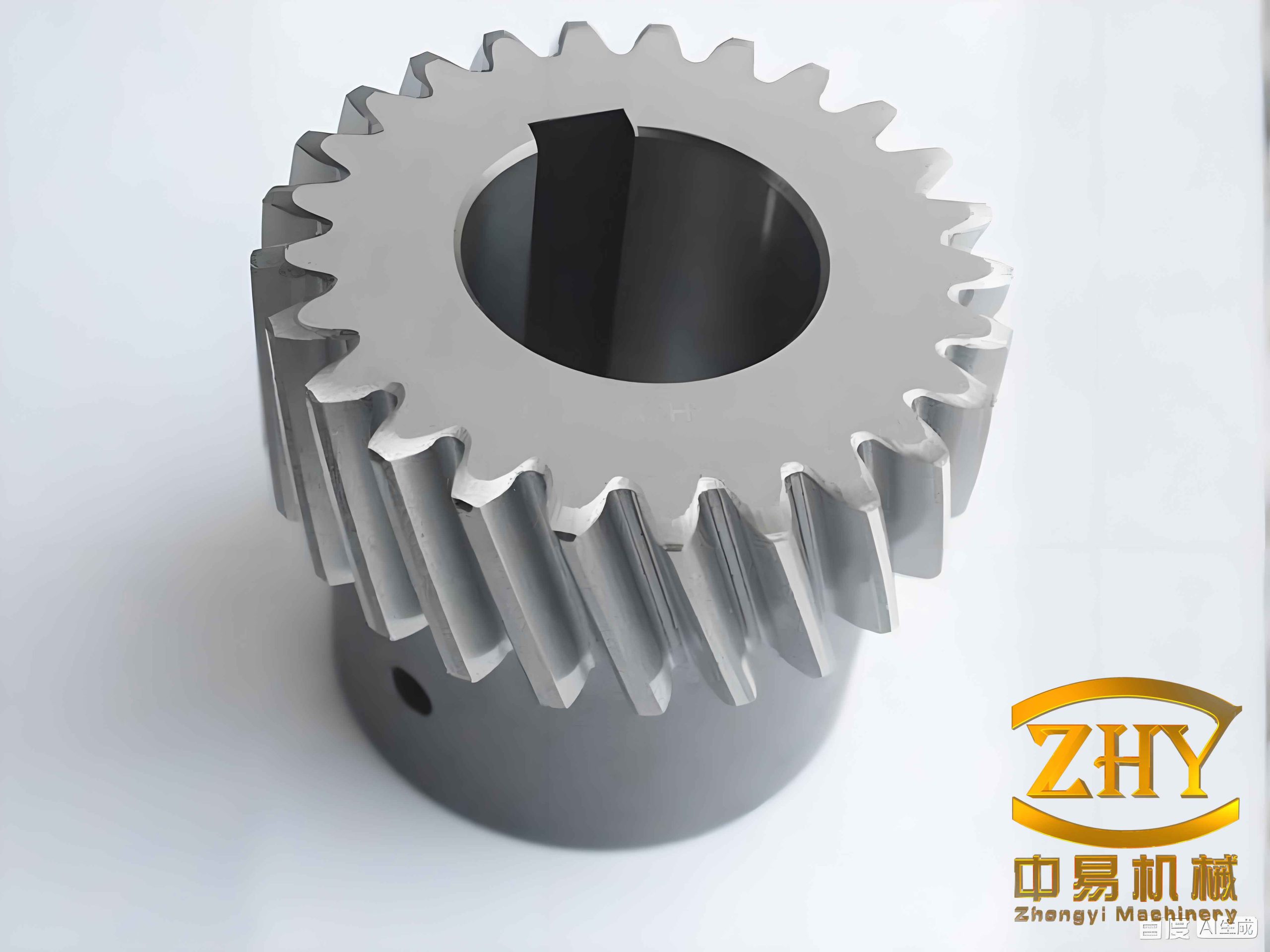
I define the relative displacement of the helical gears along the normal mesh direction as
$$
p=(Y_1-Y_2)\sin\beta-(Z_1-Z_2)\cos\beta-(r_1\theta_1-r_2\theta_2)-e(t),
$$
where \(\beta\) is the helix angle, \(r_1\) and \(r_2\) are the base radii, and \(e(t)\) is the comprehensive transmission error. The backlash function is
$$
f(p,b)=
\begin{cases}
p-b, & p>b,\\
0, & |p|\le b,\\
p+b, & p<-b,
\end{cases}
$$
where \(b\) is half of the backlash. The time-varying mesh stiffness of the helical gears is represented by
$$
K_h(t)=k_m\left[1+\varepsilon\cos(\Omega_h t)\right],
$$
where \(k_m\) is the mean mesh stiffness, \(\varepsilon\) is the stiffness fluctuation coefficient, and \(\Omega_h\) is the mesh frequency. The comprehensive transmission error is expressed as a finite Fourier series:
$$
e(t)=\sum_{\ell=1}^{N_e}A_{e\ell}\cos(\ell\Omega_e t+\Phi_\ell).
$$
The dynamic normal mesh force is
$$
F_n=K_h(t)f(p,b)+C_h\dot p,
$$
and its transverse components are
$$
F_y=F_n\cos\beta,\qquad F_z=F_n\sin\beta.
$$
Using Newton’s second law, I obtain the coupled equations of motion for the helical gears as
$$
\begin{aligned}
m_1\ddot Y_1+C_{1y}\dot Y_1+k_{1y}Y_1 &= F_y,\\
m_1\ddot Z_1+C_{1z}\dot Z_1+k_{1z}Z_1 &= F_z,\\
I_1\ddot\theta_1 &= T_1-F_n r_1,\\
m_2\ddot Y_2+C_{2y}\dot Y_2+k_{2y}Y_2 &= -F_y,\\
m_2\ddot Z_2+C_{2z}\dot Z_2+k_{2z}Z_2 &= -F_z,\\
I_2\ddot\theta_2 &= -T_2+F_n r_2.
\end{aligned}
$$
After nondimensionalization, I write the system as a ten-dimensional state equation:
$$
\dot x_1=x_2,
$$
$$
\dot x_2=-2\zeta_{11}x_2-k_{11}x_1+c_\beta\lambda k_h f(x_9,b)+c_\beta\lambda\zeta_{31}x_{10},
$$
$$
\dot x_3=x_4,
$$
$$
\dot x_4=-2\zeta_{21}x_4-k_{21}x_3+c_\beta\lambda k_h f(x_9,b)+c_\beta\lambda\zeta_{31}x_{10},
$$
$$
\dot x_5=x_6,
$$
$$
\dot x_6=-2\zeta_{12}x_6-k_{12}x_5+c_\beta\lambda k_h f(x_9,b)+c_\beta\lambda\zeta_{32}x_{10},
$$
$$
\dot x_7=x_8,
$$
$$
\dot x_8=-2\zeta_{22}x_8-k_{22}x_7+c_\beta\lambda k_h f(x_9,b)+c_\beta\lambda\zeta_{32}x_{10},
$$
$$
\dot x_9=x_{10},
$$
$$
\dot x_{10}=-c_1x_2-c_2x_4-c_1x_6-c_2x_8-\zeta_{33}x_{10}-k_h c_\lambda f(x_9,b)+f_{pm}+f_{pv}+f_e.
$$
Here \(x_9\) is the dimensionless relative displacement of the helical gears, \(x_{10}\) is its velocity, \(\Omega\) is the dimensionless mesh frequency, \(f_{pm}\) is the constant load coefficient, \(f_{pv}\) is the fluctuating load coefficient, and \(f_e\) is the transmission error excitation coefficient. The nonlinearity of the helical gears is concentrated in the backlash function \(f(x_9,b)\), the time-varying stiffness \(k_h\), and the transmission error \(f_e\).
| Symbol | Meaning in the helical gear model | Role |
|---|---|---|
| \(Y_i,Z_i\) | Transverse displacements of gear \(i\) | Couples bending and axial motion |
| \(\theta_i\) | Rotation of gear \(i\) | Transfers torque through mesh |
| \(\beta\) | Helix angle | Couples transverse directions |
| \(b\) | Half backlash | Introduces piecewise nonlinearity |
| \(K_h(t)\) | Time-varying mesh stiffness | Parametric excitation |
| \(e(t)\) | Comprehensive transmission error | Internal displacement excitation |
| \(F_n\) | Normal dynamic mesh force | Drives vibration of helical gears |
| \(\Omega\) | Dimensionless mesh frequency | Main bifurcation parameter |
| \(f_{pm}\) | Constant load coefficient | Controllable load parameter |
3. Numerical Tools for Helical Gears
I use several nonlinear dynamic indicators to identify the motion state of helical gears. A phase portrait shows whether the orbit is closed. A bifurcation diagram shows how the number of solution branches changes with a parameter. A Lyapunov exponent diagram provides a quantitative criterion for chaos. A Poincare section reduces the continuous orbit to discrete points and therefore distinguishes period-one, period-two, quasi-periodic, and chaotic motion of helical gears.
For the impact state of helical gears, I define the minimum mesh error \(x_{\min}\). The impact code is
$$
\text{impact}=
\begin{cases}
0, & x_{\min}>b,\\
1, & x_{\min}=b,\\
2, & x_{\min}<b. $$=""
The contact-loss duty ratio and back-side mesh ratio are
$$
DC_1=\frac{t_1}{T},\qquad DC_2=\frac{t_2}{T},
$$
where \(t_1\) is the contact-loss time in one mesh period \(T\), and \(t_2\) is the back-side mesh time. The dynamic load coefficient is
$$
DLC=\frac{\max\left(\sum_{i=1}^{3}k_i(\tau)f(x_i,b)+\sum_{i=1}^{3}\zeta_i x_i\right)}{f_m}.
$$
The maximum Lyapunov exponent is estimated by
$$
\lambda_{\max}=\lim_{n\to\infty}\frac{1}{n}\sum_{n_0=1}^{n}\ln\left|\frac{df(x_n,\mu)}{dx}\right|.
$$
| Tool | What I observe | Interpretation for helical gears |
|---|---|---|
| Phase portrait | Shape and number of closed curves | Periodic or non-periodic orbit |
| Poincare section | Discrete points | One point: P1; several points: Pn; closed curve: quasi-periodic; cloud: chaos |
| Bifurcation diagram | Branches versus parameter | Period-doubling, saddle-node, inverse bifurcation |
| Lyapunov exponent | Sign of \(\lambda_{\max}\) | Positive value indicates chaos in helical gears |
| Impact code | 0, 1, or 2 | No impact, single-sided impact, double-sided impact |
| Duty ratios | \(DC_1\), \(DC_2\) | Severity of contact loss and back-side contact |
| Dynamic load coefficient | DLC | Amplification of dynamic tooth load |
4. Effects of Nonlinear Factors on Helical Gears
I solve the state equations with a fourth- and fifth-order Runge-Kutta method. I then construct two-parameter diagrams in the mesh-frequency and load-coefficient plane. In these diagrams, each small cell represents a possible motion state, and the color indicates impact state, period number, contact-loss ratio, back-side contact ratio, or dynamic load coefficient. This approach allows me to compare how different nonlinear factors affect the behavior of helical gears.
4.1 Time-varying mesh stiffness
I compare two stiffness fluctuation coefficients, \(\varepsilon=0.1\) and \(\varepsilon=0.25\). When \(\varepsilon\) increases, the chaotic region of helical gears decreases significantly. The no-impact region increases, and the P2, P4, and P8 periodic regions expand. The contact-loss duty ratio also decreases. Therefore, a larger time-varying mesh stiffness coefficient tends to make the motion of helical gears smoother, although the dynamic load coefficient may still increase in some local regions.
| Quantity | \(\varepsilon=0.1\) | \(\varepsilon=0.25\) | Trend for helical gears |
|---|---|---|---|
| Chaotic area share | 49.6% | 9.0% | Decreases strongly |
| No-impact area share | 2.4% | 5.4% | Increases |
| P2 area | Baseline | +18% | Periodic region expands |
| P4 area | Baseline | +1.9% | Periodic region expands |
| P8 area | Baseline | +6.5% | Periodic region expands |
| Contact-loss duty ratio | Higher in some ranges | Lower overall | Impact is relieved |
4.2 Comprehensive transmission error
I compare \(f_e=0.01\) and \(f_e=0.05\). As the comprehensive transmission error increases, the chaotic area of helical gears grows from about 9.0% to about 50.4%. The P2 motion share decreases from 35.4% to 13.0%, and the P4, P8, and P16 shares also decrease. The contact-loss duty ratio increases, and the dynamic load coefficient increases. Thus, a larger transmission error makes the motion of helical gears less regular and increases contact loss and dynamic load.
| Quantity | \(f_e=0.01\) | \(f_e=0.05\) | Trend for helical gears |
|---|---|---|---|
| Chaotic area share | 9.0% | 50.4% | Increases strongly |
| P1/1 area share | 32.5% | 35.8% | Relatively stable |
| P2 area share | 35.4% | 13.0% | Decreases |
| P4, P8, P16 share | 17.6% | 1.1% | Decreases |
| Contact-loss duty ratio | Lower | Higher | Worsens |
| Dynamic load coefficient | 1.0 to 1.02 | Above 1.0 with wider range | Increases |
4.3 Backlash
I compare \(b=0.014\) and \(b=1\). A very small backlash can cause back-side contact, while a larger backlash removes double-sided impact in the studied range. When \(b=1\), the double-sided impact region disappears, and the chaotic single-sided impact region expands. The back-side mesh ratio is zero for the larger backlash case, but for the small backlash case, non-zero back-side contact appears in several regions. Therefore, backlash has a strong influence on the back-side contact of helical gears, and an excessively small backlash may worsen tooth back contact.
| Quantity | \(b=0.014\) | \(b=1\) | Trend for helical gears |
|---|---|---|---|
| Double-sided impact | 17.5% area | Disappears | Reduced by larger backlash |
| P2 area share | 31.8% | 35.4% | Increases |
| P4, P8, P16 share | 9.2% | 17.6% | Increases |
| Back-side mesh ratio | Non-zero in several zones | Zero in studied range | Small backlash aggravates back-side contact |
| Dynamic load coefficient | Some lower range | Some higher range | Depends on load and frequency |
5. Bifurcation Characteristics of Helical Gears
I choose the dimensionless mesh frequency \(\Omega\) as the main bifurcation parameter. As \(\Omega\) increases, the helical gears undergo a sequence of transitions. In one parameter set, the motion changes from period-one to period-two through a saddle-node bifurcation, then to period-four and period-eight through period-doubling, and finally to chaos. Inside the chaotic region, periodic windows appear. At higher frequencies, inverse period-doubling brings the system back to period-eight, period-four, period-two, and finally period-one. This route is important for helical gears because it shows that chaos is not isolated but is embedded in a sequence of periodic and chaotic windows.
| Parameter range | Observed motion of helical gears | Bifurcation type |
|---|---|---|
| \(\Omega\in[1.15,1.173]\) | Period-one | Stable periodic motion |
| \(\Omega\approx1.173\) | P1 to P2 | Saddle-node bifurcation |
| \(\Omega\in[1.173,1.2338]\) | Period-two | Periodic motion |
| \(\Omega\approx1.2327\) | P2 to P4 | Period-doubling |
| \(\Omega\in[1.234,1.236]\) | P8 to chaos | Period-doubling route |
| \(\Omega\in[1.236,1.336]\) | Chaos with periodic windows | Chaotic vibration |
| \(\Omega\approx1.339\) | P8 | Inverse period-doubling |
| \(\Omega\approx1.3438\) | P4 | Inverse period-doubling |
| \(\Omega\approx1.3536\) | P2 | Inverse period-doubling |
| \(\Omega\approx1.4137\) | P1 | Stable periodic motion |
I also use the load coefficient \(f_{pm}\) as a bifurcation parameter. In one case, as \(f_{pm}\) increases, the helical gears first undergo period-doubling from period-one to period-two and then to chaos. For larger \(f_{pm}\), inverse period-doubling returns the motion to period-four, period-two, and period-one. This confirms that the load level of helical gears can be used as a control parameter to shift the system away from chaos.
| Load range | Motion of helical gears | Behavior |
|---|---|---|
| \(f_{pm}\in[0,0.006]\) | P1, P2, then chaos | Period-doubling to chaos |
| \(f_{pm}\in[0.006,0.0136]\) | Chaotic vibration | Undesirable motion |
| \(f_{pm}\in[0.0136,0.03]\) | P4, P2, P1 | Inverse period-doubling |
In the two-parameter plane of mesh frequency and load coefficient, I identify regions of chaotic and periodic motion. This plane is useful because a single perturbation may be insufficient to control helical gears when the desired periodic orbit lies far from the current parameter point. Simultaneous perturbation of mesh frequency and load coefficient can reduce the required perturbation amplitude and improve controllability.
| Region | Initial state of helical gears | Target state | Control implication |
|---|---|---|---|
| K1 to K2 | Chaos | Period-one | Both parameters can be perturbed |
| K3 to K4 | Chaos | Period-two | Single-parameter control may need large amplitude |
| K5 to K6 | Chaos | Period-four | Two-parameter control is preferred |
6. Neural Network Controller Design for Helical Gears
I design two controllers for the helical gears: a radial basis function neural network controller and a back-propagation neural network controller. The controller input is formed from distances between adjacent points on the Poincare section. If \(X(k)\) is the point at the \(k\)-th iteration, I define
$$
d(k)=\|X(k)-X(k-1)\|,
$$
and the controller input vector is
$$
D(k)=[d(k-1),d(k)].
$$
The desired distance on the Poincare section is \(d^*\), which is chosen as the smallest positive floating-point separation that can be distinguished numerically. The control error is
$$
e(k)=d^*-d(k).
$$
For the radial basis function neural network, I use a Gaussian basis. The controller output is
$$
u(k)=\sum_{j=1}^{m}\omega_j\exp\left(-\frac{\|D(k)-c_j\|^2}{2b_j^2}\right),
$$
where \(\omega_j\) is the output weight, \(c_j\) is the center of the \(j\)-th basis function, and \(b_j\) is its width. I use two input nodes, five hidden nodes, and one output node. The search ranges are
$$
\omega_j\in[-1,1],\qquad b_j\in[0.1,1],\qquad c_j\in[-1,1].
$$
For the back-propagation neural network, I use a sigmoid activation function. The hidden layer output is
$$
h_j=\sigma\left(\sum_{i=1}^{2}w_{ij}^{(1)}D_i(k)+b_j^{(1)}\right),
$$
and the controller output is
$$
u(k)=\sum_{j=1}^{5}w_j^{(2)}h_j+b^{(2)}.
$$
The fitness function for the optimization algorithm is
$$
fit_i(t)=\sum_{k=1}^{L}\left|\|X(k)-X(k-1)\|-d^*\right|.
$$
This fitness function connects the improved gravitational search algorithm to the neural network controller. Because the distance between adjacent Poincare points should be as close as possible to \(d^*\), a smaller fitness value means that the controller has driven the helical gears closer to the desired periodic orbit.
| Item | RBF controller | BP controller |
|---|---|---|
| Input nodes | 2 | 2 |
| Hidden nodes | 5 | 5 |
| Output nodes | 1 | 1 |
| Basis or activation | Gaussian radial basis | Sigmoid |
| Optimized parameters | \(\omega_j,c_j,b_j\) | \(w_{ij}^{(1)},b_j^{(1)},w_j^{(2)},b^{(2)}\) |
| Search range for weights | \([-1,1]\) | \([-10,10]\) |
| Search range for bias or width | \(b_j\in[0.1,1]\) | \(b\in[-1,1]\) |
The control procedure is as follows. I first let the helical gears evolve for a fixed number of iterations to obtain the initial Poincare distances. Then I initialize the improved gravitational search algorithm. For each candidate parameter set, I apply the neural network controller to the helical gears and measure the resulting Poincare distances. I update the particle positions until the maximum number of iterations is reached. The best parameter set is then used to control the helical gears. The output perturbation is constrained by a maximum allowable value, so the controller remains a small-perturbation controller.
| Step | Operation | Purpose for helical gears |
|---|---|---|
| 1 | Compute initial Poincare distances | Provide controller input |
| 2 | Initialize improved GSA population | Set controller parameter candidates |
| 3 | Map each particle to controller parameters | Evaluate control performance |
| 4 | Apply perturbation \(u(k)\) | Drive helical gears toward target orbit |
| 5 | Measure new Poincare distances | Update controller input |
| 6 | Compute fitness | Rank particles |
| 7 | Update particle positions | Search better controller parameters |
| 8 | Output best parameters | Control chaotic helical gears |
7. Improved Gravitational Search Algorithm
The gravitational search algorithm treats each candidate solution as a particle with mass. The mass of a particle is determined by its fitness. Heavier particles attract lighter particles, so the population moves toward better regions. For controller optimization in helical gears, the algorithm must be accurate because chaotic systems are highly sensitive to small perturbations. The standard gravitational search algorithm has strong global search ability but weak local exploitation and can easily become trapped in local optima. I therefore improve the initialization, memory, attenuation factor, inertial mass, and local search.
In the standard algorithm, the inertial mass is
$$
M_i(t)=\frac{m_i(t)}{\sum_{j=1}^{N}m_j(t)},
$$
where
$$
m_i(t)=\frac{fit_i(t)-worst(t)}{best(t)-worst(t)}.
$$
The gravitational force acting on particle \(i\) in dimension \(d\) is
$$
F_{ij}^d(t)=G(t)\frac{M_i(t)M_j(t)}{R_{ij}(t)+\epsilon}\left(x_j^d(t)-x_i^d(t)\right),
$$
and the total force is
$$
F_i^d(t)=\sum_{j=1,j\ne i}^{N}\operatorname{rand}_jF_{ij}^d(t).
$$
The acceleration, velocity, and position updates are
$$
a_i^d(t)=\frac{F_i^d(t)}{M_i(t)},
$$
$$
v_i^d(t+1)=\operatorname{rand}_i v_i^d(t)+a_i^d(t),
$$
$$
x_i^d(t+1)=x_i^d(t)+v_i^d(t+1).
$$
The gravitational constant is
$$
G(t)=G_0e^{-\alpha t/T}.
$$
My improvements are summarized below.
| Improvement | Method | Effect on helical gear control |
|---|---|---|
| Initialization | Sobol sequence | Improves coverage and diversity of controller parameters |
| Particle memory | Use personal best and global best | Prevents oscillation near a local optimum |
| Adaptive attenuation | Use time-dependent \(\alpha(t)\) | Large step early, small step late |
| Weighted inertial mass | Add a weight factor to \(M_i(t)\) | Amplifies differences between particles |
| Chaotic local search | Piecewise chaotic map | Improves final accuracy for chaotic helical gears |
For the memory term, I use
$$
V(t+1)=\operatorname{rand}_1V(t)+a+c_1\operatorname{rand}_2(qbest-X(t))+c_2\operatorname{rand}_3(gbest-X(t)),
$$
where \(qbest=Y Lbest(t)\), \(Y\) is a matrix of ones, and \(Lbest(t)\) is the current global best. The coefficients are chosen as
$$
c_1=1-\left(\frac{t}{T}\right)^3,\qquad c_2=1+\left(\frac{t}{T}\right)^3.
$$
Thus, the global best has a larger influence in the later stage, while the early stage keeps a broader search. For the attenuation factor, I use
$$
\alpha(t)=\alpha_0\frac{t}{T}.
$$
For the weighted inertial mass, I use
$$
MG_i(t)=M_i(t)+\frac{1}{\ln(t+10)}\omega_i(t)M_i(t),
$$
where \(\omega_i(t)\) is a weight determined by the maximum and minimum masses. For the chaotic search, I use the Piecewise map:
$$
x(t+1)=
\begin{cases}
\dfrac{x(t)}{p}, & 0\le x(t)<p,\\[6pt] $$="" &="" 0.5\le="" 1-\dfrac{1-x(t)}{p},="" 1-\dfrac{x(t)-0.5}{p},="" 1-p\le="" <p="" \dfrac{x(t)-p}{0.5-p},="" \end{cases}="" p\le="" x(t)<0.5,\\[6pt]="" x(t)<1-p,\\[6pt]="" x(t)I test the improved algorithm on several multimodal functions. The test functions include Griewank, Rastrigin, Ackley, Schaffer, and Alpine functions. I set the dimension to 30 and the maximum iteration number to 2000. The improved algorithm escapes local optima more often and reaches a lower final value than the standard algorithm.
| Test function | Range | Global minimum | Observed improvement |
|---|---|---|---|
| Griewank | \([-600,600]^n\) | 0 | Better final accuracy |
| Rastrigin | \([-5,5]^n\) | 0 | Less premature convergence |
| Ackley | \([-32,32]^n\) | 0 | Stronger local exploitation |
| Schaffer | \([-100,100]^n\) | 0 | Faster escape from local basins |
| Alpine | \([-10,10]^n\) | 0 | More stable convergence |
8. Chaos Control Simulations for Helical Gears
I apply the designed controllers to the six-degree-of-freedom helical gear system. In each case, the controller is activated after an initial transient. The perturbation is applied to either the mesh frequency or the load coefficient, or to both. I compare the radial basis function controller and the back-propagation controller in terms of control speed, final orbit, and perturbation amplitude.
8.1 Inverse period-doubling interval
In the inverse period-doubling interval, the helical gears exhibit chaotic motion before control. The radial basis function controller and the back-propagation controller both drive the system to period-one, period-two, and period-four orbits. For period-one and period-two, the two controllers require about the same number of control cycles and the final orbits are nearly identical. For period-four, the radial basis function controller produces a smaller perturbation amplitude. Overall, the two controllers perform similarly in this interval, but the radial basis function controller is slightly more efficient in perturbation size.
| Target orbit | Initial motion of helical gears | RBF control cycles | BP control cycles | Preferred controller |
|---|---|---|---|---|
| Period-one | Chaos | Short | Short | Comparable |
| Period-two | Chaos | Short | Short | RBF has smaller perturbation |
| Period-four | Chaos | About 5 | About 5 | RBF |
8.2 Saddle-node bifurcation interval
In the saddle-node interval, the helical gears also exhibit chaos, but the bifurcation structure differs from the inverse period-doubling case. I target period-one motion. Both controllers complete the transition within about forty control cycles. The final orbits are the same, but the back-propagation controller requires a larger perturbation range than the radial basis function controller. Therefore, the radial basis function controller is preferred for the saddle-node interval of helical gears.
| Target orbit | Initial motion of helical gears | Control speed | Perturbation amplitude | Preferred controller |
|---|---|---|---|---|
| Period-one | Chaos | Within about 40 cycles | BP larger | RBF |
8.3 Multi-period interval
In the multi-period interval, the helical gears move on a multi-periodic orbit before control. I drive them to period-one, period-two, and period-four. The radial basis function controller reaches period-one in about ten control cycles, while the back-propagation controller needs about twenty cycles. For period-two and period-four, both controllers reach the target in about ten cycles. The final orbits may differ slightly because the optimization searches different valid parameter sets. In general, the radial basis function controller uses smaller or comparable perturbations. I also control a period-four helical gear system to period-two and period-one. The transition is completed in about ten cycles, and the two controllers produce similar final orbits.
| Initial orbit | Target orbit | RBF speed | BP speed | Perturbation comparison |
|---|---|---|---|---|
| Multi-period | Period-one | About 10 cycles | About 20 cycles | RBF smaller |
| Multi-period | Period-two | About 10 cycles | About 10 cycles | RBF larger in one case |
| Multi-period | Period-four | About 10 cycles | About 10 cycles | RBF smaller |
| Period-four | Period-one | About 10 cycles | About 10 cycles | BP smaller |
| Period-four | Period-two | About 10 cycles | About 10 cycles | RBF larger |
8.4 Quasi-periodic interval
In the quasi-periodic interval, the Poincare section of the helical gears is a closed curve rather than a cloud of points. The radial basis function controller and the back-propagation controller both drive the system to period-one and period-three. For period-one, the radial basis function controller converges in about forty cycles, while the back-propagation controller requires at least sixty cycles. The perturbation ranges are similar. For period-three, the radial basis function controller also performs better, although its perturbation amplitude is somewhat larger. Thus, the radial basis function controller is more suitable for quasi-periodic helical gears.
| Target orbit | Initial motion of helical gears | RBF convergence | BP convergence | Preferred controller |
|---|---|---|---|---|
| Period-one | Quasi-periodic | About 40 cycles | At least 60 cycles | RBF |
| Period-three | Quasi-periodic | Faster | Slower | RBF |
8.5 Load bifurcation interval
I also use the load coefficient as the control parameter. In the chaotic interval of the load bifurcation diagram, the radial basis function and back-propagation controllers drive the helical gears to period-one, period-two, and period-four. The perturbation ranges and control speeds are similar. For period-one, the radial basis function controller uses a smaller parameter perturbation, so it is preferred. For period-two and period-four, the two controllers perform almost equally.
| Target orbit | Control parameter | Initial motion of helical gears | RBF performance | BP performance |
|---|---|---|---|---|
| Period-one | Load coefficient | Chaos | Smaller perturbation | Larger perturbation |
| Period-two | Load coefficient | Chaos | Comparable | Comparable |
| Period-four | Load coefficient | Chaos | Comparable | Comparable |
8.6 Two-parameter control in the mesh-frequency and load plane
Because a single perturbation may be insufficient for some regions of the mesh-frequency and load plane, I design a parallel radial basis function controller. Two radial basis function networks share the same distance inputs, but one network outputs a perturbation to the mesh frequency and the other outputs a perturbation to the load coefficient. This controller can simultaneously adjust two controllable parameters of the helical gears. I test three transitions: chaos to period-one, chaos to period-two, and chaos to period-four. In each case, the parallel controller drives the helical gears to the target orbit. The perturbations settle to steady values, and the system reaches the desired periodic state.
| Transition | Initial motion of helical gears | Target orbit | Mesh-frequency perturbation | Load perturbation |
|---|---|---|---|---|
| K1 to K2 | Chaos | Period-one | Active then steady | Active then steady |
| K3 to K4 | Chaos | Period-two | Becomes near zero | Steady non-zero |
| K5 to K6 | Chaos | Period-four | Persistent small value | Persistent small value |
9. Discussion
The numerical results reveal several important features of helical gears. First, chaotic vibration is not confined to a narrow parameter range. It appears in the mesh-frequency interval, the load interval, and the two-parameter plane. Second, the route to chaos depends on the parameter direction. Period-doubling, inverse period-doubling, and saddle-node bifurcation can all be observed. Third, the nonlinear factors of helical gears have different effects: time-varying mesh stiffness tends to reduce chaos, transmission error tends to increase chaos, and backlash mainly affects back-side contact. Fourth, neural network control is effective even though the exact Jacobian matrix of the helical gears is not used. The controller only needs the distances between adjacent Poincare points, which reduces the computational burden and avoids the eigenvalue sensitivity problem of OGY-type methods in high-dimensional systems.
The radial basis function controller performs better than the back-propagation controller in most cases. The reason is that the Gaussian radial basis can localize the response in the input space, and the optimized centers and widths allow the controller to fit the nonlinear relationship between Poincare distance and required perturbation. The back-propagation controller can also drive helical gears to periodic orbits, but it often requires larger perturbations or more control cycles. The improved gravitational search algorithm plays a central role because it finds controller parameters that are accurate enough for chaotic helical gears. The Sobol initialization improves population coverage, the memory term reduces oscillation near local optima, the adaptive attenuation factor balances exploration and exploitation, the weighted inertial mass increases particle diversity, and the chaotic search refines the final solution.
| Observation | Implication for helical gears |
|---|---|
| Chaos appears in multiple parameter intervals | Control design must be robust over a wide operating range |
| Periodic windows exist inside chaos | Small perturbations can target nearby periodic orbits |
| Transmission error increases chaos | High manufacturing and assembly accuracy is beneficial |
| Small backlash increases back-side contact | Backlash selection must consider contact loss and back-side impact |
| RBF controller generally performs better | Gaussian RBF is suitable for nonlinear control of helical gears |
| Two-parameter control expands controllability | Mesh frequency and load can be adjusted together |
10. Conclusion
I have established a six-degree-of-freedom nonlinear dynamic model of helical gears and analyzed its chaotic vibration under time-varying mesh stiffness, comprehensive transmission error, backlash, damping, and load. I used two-parameter diagrams, bifurcation diagrams, phase portraits, and Poincare sections to identify periodic, quasi-periodic, multi-periodic, and chaotic motion. I designed radial basis function and back-propagation neural network controllers and optimized their parameters with an improved gravitational search algorithm. The improved algorithm uses Sobol initialization, memory-based velocity update, adaptive attenuation, weighted inertial mass, and Piecewise chaotic search. I then controlled chaotic, quasi-periodic, and multi-periodic helical gears by perturbing mesh frequency, load coefficient, or both. The radial basis function controller generally achieves faster convergence and smaller perturbations than the back-propagation controller. The two-parameter radial basis function controller successfully drives helical gears from chaos to period-one, period-two, and period-four in the mesh-frequency and load plane. The results provide a useful numerical basis for suppressing chaotic vibration in helical gears and for improving the operational stability of geared transmission systems.
| Contribution | Outcome for helical gears |
|---|---|
| Six-degree-of-freedom nonlinear model | Captures coupled transverse, axial, and torsional behavior |
| Two-parameter maps | Reveal impact, contact-loss, back-side contact, and dynamic load regions |
| Bifurcation analysis | Identifies chaotic, quasi-periodic, and multi-periodic intervals |
| RBF and BP controllers | Drive helical gears to prescribed periodic orbits |
| Improved GSA | Provides accurate controller parameters for chaotic helical gears |
| Two-parameter control | Handles regions where single-parameter control is insufficient |
For future work, I would extend the model of helical gears by including more nonlinear effects such as friction, thermal deformation, bearing clearance, and time-varying support stiffness. I would also perform experimental validation on a gearbox test rig to compare with the numerical results. These extensions would further improve the reliability of chaos control for helical gears in practical transmission systems.